Keywords: Spark, BFS, Shortest Path, Betweenness centrality, Text Analysis

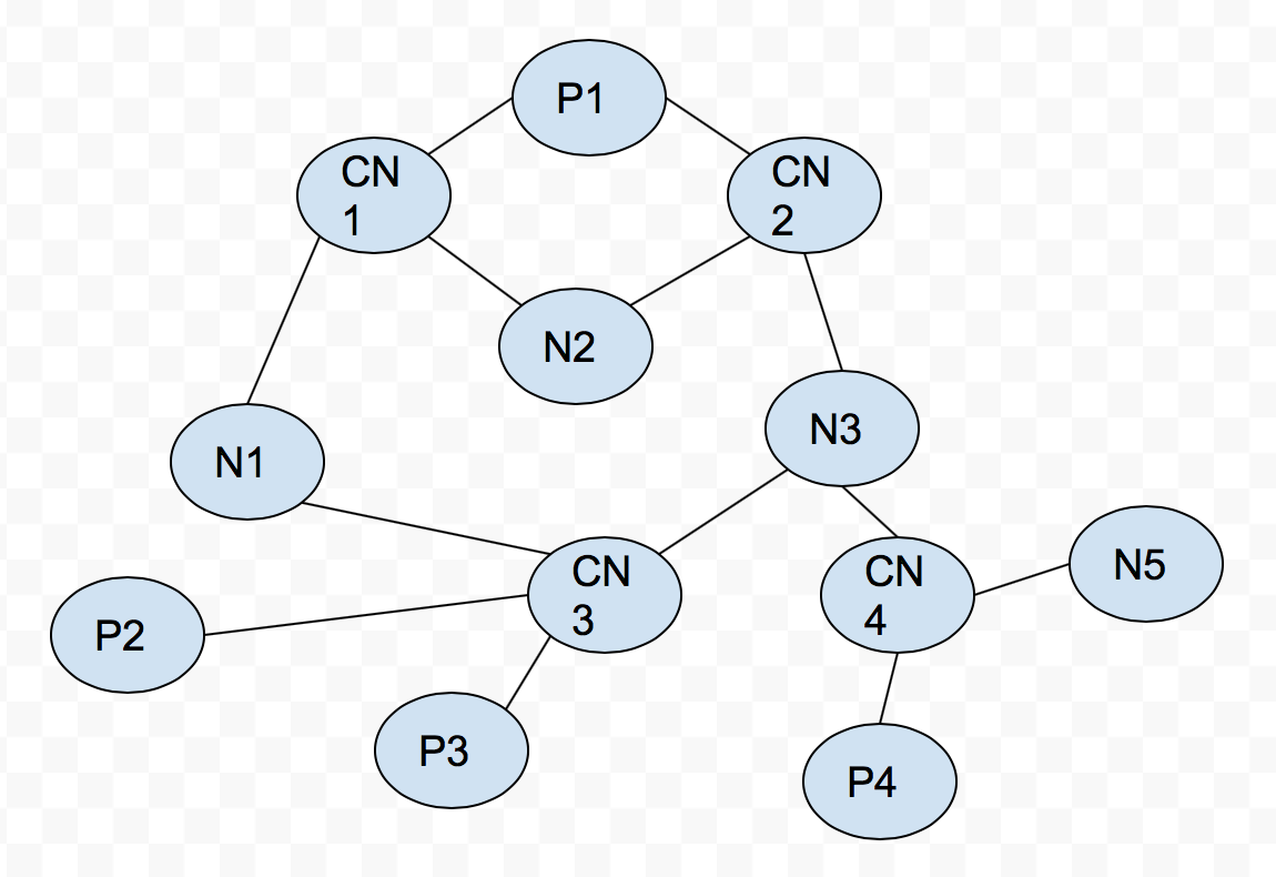
P means paper node, CN is compound nouns node, N is noun node.

class Node {
    long id,
    Map sourceId -> (distance, sigma, precedence[count])
}

Betweenness centrality is an indicator of a node's centrality in a network. It is equal to the number of shortest paths from all vertices to all others that pass through that node. A node with high betweenness centrality has a large influence on the transfer of items through the network, under the assumption that item transfer follows the shortest paths.

where σ s,t is the number of shortest (s, t)-paths, and σ s,t (v) is the number of those paths passing through some node v other than s, t. If s = t, σ s,t = 1, and if v in {s, t}, σ s,t (v) = 0

Ulrik Brandes has proposed a algorithm to decrease the complextity of O(n^3) to O(mn) for unweighted graph, but its sequencial algorithm. So we finally implement the algorithm proposed by David A. Bader, which still be O(n^3) complexity but can be implemented in paralle mode. Assume a graph G = (V,E), n is the number of vertices, and m is the number of edges. The main idea of the algorithm is to perform n breadth-first graph traversals and augment each traversal to compute the number of shortest paths passing through each vertex. We store a multiset P of predecessors associated with each vertex. Here, a vertex belongs to the predecessor multiset of w if

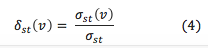
where, d(s, v) shortest path from source vertex s to vertex v. The predecessor information is used in the dependency accumulation step (step III in Algorithm). Here we introduce the dependency value as

where, δst (v) is the pairwise dependencies of vertices s and v.

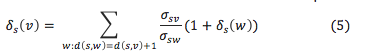
Given the information of predecessors of each vertex, we can get the dependency values δs (v) without the need to traverse all the other vertices. The new equation is:

The algorithm is below:

Algorithm
Input: G(V, E)
Output: BC[1...n], where BC[v] gives the	 centrality score for vertex.
1: for all v ∈ V in parallel do
2: 		BC[v] ← 0
3: for all s ∈ V do
	I. Initialization
4: for all t ∈ V in parallel do
5: 		P[t] ← empty multiset, σ[t] ← 0, d[t] ← -1
6:	σ[s] ← 1, d[s] ← 0
7: phase ← 0, S[phase] ← empty stack
8: push s → S[phase]
9: count ← 1
	II. Graph traversal for shortest path discovery and counting
10:	while count > 0 do
11:		count ← 0
12:		for all v ∈ S[phase] in parallel do
13:			for each neighbor w of v in parallel do
14:				if d[w] < 0 then
15:					push w → S[phase+1]
16:					count ← count + 1
17:					d[w] ← d[v] + 1
18:				if d[w] = d[v] + 1 then
19:					 σ[w] ← σ[w] + σ[v]
20:					 append v → P[w]
21:			phase ← phase + 1
22:		phase ← phase - 1
	III. Dependency accumulation by back-propagation
23:	δ[t] ← 0 ∀ t ∈ V
24:	while phase > 0 do
25:		for all w ∈ S[phase] in parallel do
26:			for all v ∈ P[w] do
27:				δ[v] ← δ[v] + σ[v]/σ[w] * (1+δ[w])
28:			BC[w] ← BC[w] + δ[w]
29:		phase ← phase - 1

We test the program on CCR HPC in SUNY Buffalo. The data is from PubMed.

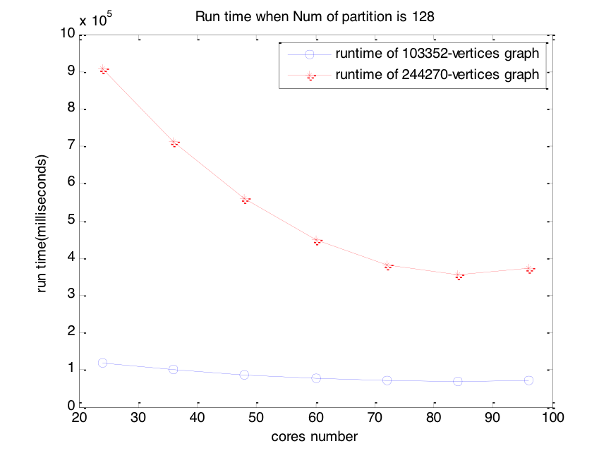
Based on the CCR system, we compute approximate betweenness centrality for graphs of 103,352 vertices and 244,270 vertices on cores which size range from 24 cores to 96 cores with 128 partitions and 258 partitions.

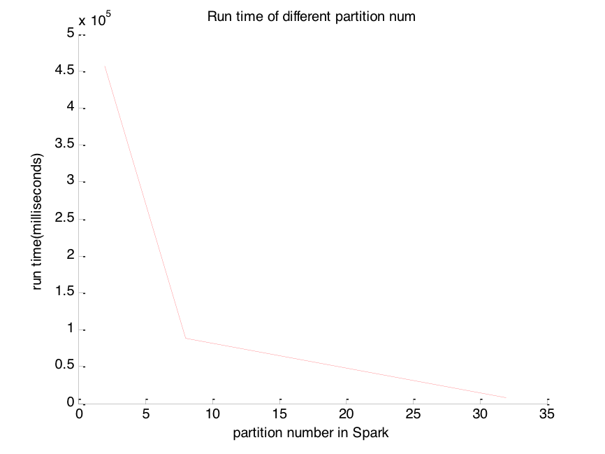
The running efficiency of Spark will be affected by partition number of data. Then we test on a sample data with total 24 cores, as we can see, when we set the number of the partition to be above a threshold, the runtime efficiency would be dramatically improved.

Firstly we implement the algorithm on a workload of 103352 vertices graph and start from 24 cores to 96 cores at last. The running complexity is changing a little bit, then we can conclude the parallelization reaches the peak. Then we implement the algorithm on a workload of 244270 vertice graph, the time consumption is dramatically decreasing when we increase the parallel degree, then become stable after 64 cores.

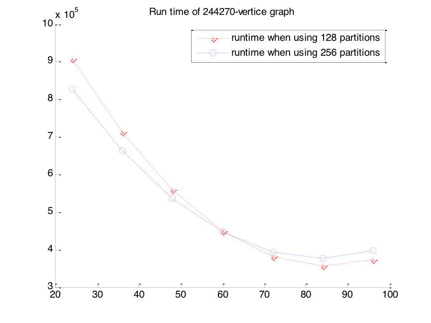
We keep the workload constant, and then we find that larger number of partitions doesn’t mean a better performance in term of runtime. As we obtain from the figure, when the number of cores is below 60, a larger amount (256) of partitions can achieve a lower total runtime. However, when the number of used cores increase to be above 60, a larger amount of partitions is no longer a good choice. Instead, a smaller (128) amount of partition may achieve a better runtime performance.

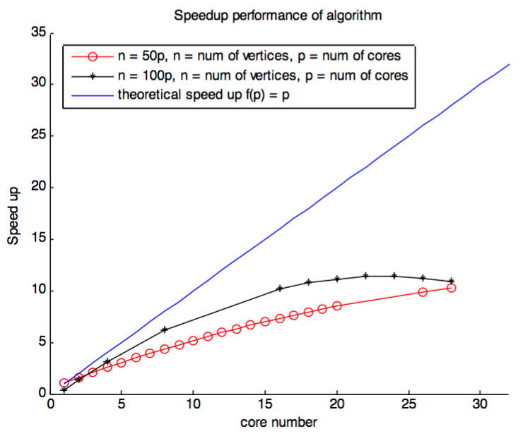
We utilized a single node to calculate the speedup performance of the similar parallel algorithm which implemented by networkx in multithread. The parallel speedup of the program running on CCR rush server is 11.4 on 24 cores for networkx. Compare to the speedup that Bader mentioned in his paper, 10.5, is increased a little bit. Consider the test machine hardware of us is much better than his, this result is quite reasonable.

1.Parallel Algorithms for Evaluating Centrality Indices in Real-world Networks, David A. Bader

2.A Faster Parallel Algorithm and Efficient Multithreaded Implementations, David A. Bader

3.A Faster Algorithm for Betweenness Centrality, Ulrik Brandes