Python tools for the filtering of digital signals.

Package management is cleanly handled on Iris via modules. The filters package has a corresponding modulefile here.

To use the filters package, change to the directory you'd like to download the source files to and retrieve the source files from github by typing

$ git clone https://github.com/emd/filters.git

The created filters directory defines the package's top-level directory. The modulefiles should be similarly cloned.

Now, at the top of the corresponding modulefile, there is a TCL variable named filters_root; this must be altered to point at the top-level directory of the cloned filters package. That's it! You shouldn't need to change anything else in the modulefile. The filters module can then be loaded, unloaded, etc., as is discussed in the above-linked Iris documentation.

The modulefile also defines a series of automated tests for the filters package. Run these tests at the command line by typing

$ test_filters

If the tests return "OK", the installation should be working.

Change to the directory you'd like to download the source files to and retrieve the source files from github by typing

$ git clone https://github.com/emd/filters.git

Change into the filters top-level directory by typing

$ cd filters

For accounts with root access, install by running

$ python setup.py install

For accounts without root access (e.g. a standard account on GA's Venus cluster), install locally by running

$ python setup.py install --user

To test your installation, run

$ nosetests tests/

If the tests return "OK", the installation should be working.

filters allows for easy digital-filter design, visualization, and application. For example, to generate a lowpass filter for a signal sampled at 100 kS/s and visualize it's amplitude response |H(f)|:

import numpy as np
import matplotlib.pyplot as plt
import filters

Fs = 1e6       # sample rate, [Fs] = samples / s
ripple = -60   # [ripple] = dB, ripple in filter's passband & stopband
width = 50e3   # [width] = Hz, width of transition between passband & stopband
f_6dB = 250e3  # [f_6dB] = Hz, (power) 6-dB frequency of filter

lpf = filters.fir.Kaiser(ripple, width, f_6dB, pass_zero=True, Fs=Fs)

df = 0.1e3    # [df] = Hz, spacing between adjacent points in response plot
lpf.plotResponse(f=np.arange(0, (0.5 * Fs) + df, df))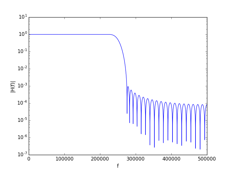

This filter can be easily applied to a given signal. For example, take the linearly chirped signal polluted by high-frequency noise below:

# Create linearly chirping signal from 10 kHz to 20 kHz.
# Note that for a linear chirp, the phase evolution goes as
# (ramp rate) * t^2, and the instantaneous frequency goes
# as 2 * (ramp rate) * t
t = np.arange(0, 0.5e-3, 1. / Fs)        # [t] = s
fstart = 10e3                          # [fstart] = Hz
fstop = 20e3                           # [fstop] = Hz
m = (fstop - fstart) / (t[-1] - t[0])  # [m] = Hz / s, chirp rate
f = fstart + (m * t)                   # frequency as function of time
y = np.cos(2 * np.pi * f * t)          # desired signal

# Corrupt signal with 400 kHz noise
y += 0.25 * np.cos(2 * np.pi * 400e3 * t)

# Apply lowpass filter to noisy signal
yfilt = lpf.applyTo(y)
valid = lpf.getValidSlice()  # points *not* corrupted by boundary effects

fig, axes = plt.subplots(2, 1, sharex=True, sharey=True)

axes[0].plot(t * 1e3, y)
axes[1].plot(t[valid] * 1e3, yfilt[valid])

# Annotate
axes[1].set_xlabel('t [ms]')
axes[0].set_title('raw')
axes[1].set_title('filtered')
axes[0].axvline(0.25, c='k', linestyle='--')
axes[1].axvline(0.25, c='k', linestyle='--')

plt.show()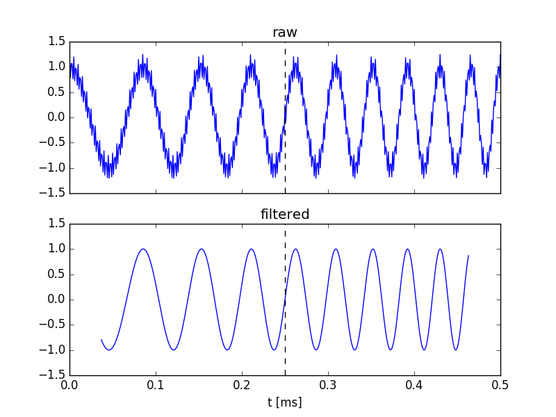

The above figure highlights several important properties of the filter:

• the 400-kHz noise has been suppressed,
• the filter imparts zero delay -- this is a generic feature of the filters produced by filters.fir.Kaiser, and
• boundary effects will plague the filtered signal -- above, the portions of the filtered signal that are plagued by boundary effects are simply not plotted.