Background:

Python tools for random data analysis.

Background:

This module (random_data) aims to provide Python tools for flexible and extensible analysis of random signals (see example use cases below). The motivation and mathematical underpinnings of this module are largely discussed in Bendat and Piersol's classic text "Random Data", and inquisitive users are directed there for a thorough discussion of the methodologies implemented in this module.

The matplotlib.mlab submodule offers several useful routines for spectral density estimation, but

psd and csd, which use Welch's average periodogram method to estimate the autospectral density and cross-spectral density, respectively, are not time-resolved, and
specgram, which creates a time-resolved estimate of the autospectral density (i.e. a "spectrogram"), does not average spectral estimates over several realizations, so the resulting spectrogram suffers from large amounts of random error

In contrast, random_data produces time-resolved spectral density estimates that have been averaged over several realizations, effectively merging the functionality of psd/csd and specgram. This is largely accomplished via class definitions built around matplotlib's psd and csd functions.

In addition, random_data provides:

a class to fit the cross-phase angles from an array of measurements to a linear model, allowing determination of mode numbers/wavenumbers as a function of frequency and time,
a class to estimate the complex-valued, spatial cross-correlation function from an array of measurements (the array need not be uniformly spaced),
a class to estimate the two-dimensional autospectral density from an array of measurements (the array need not be uniformly spaced),
robust methods for visualizing the relevant spectral estimates (magnitude, coherence, phase angle, mode number, and quality of fit),
a class for autoregressive (AR) autospectral-density estimation,
a class for "spike" identification and removal from spectral estimates, and
a class for determining the "trigger offset" between a collection of time series.

The installation and use of random_data are discussed below.

Installation:

... on GA's Iris cluster:

Package management is cleanly handled on Iris via modules. The random_data package has a corresponding modulefile here.

To use the random_data package, change to the directory you'd like to download the source files to and retrieve the source files from github by typing

$ git clone https://github.com/emd/random_data.git

The created random_data directory defines the package's top-level directory. The modulefiles should be similarly cloned.

Now, at the top of the corresponding modulefile, there is a TCL variable named random_data_root; this must be altered to point at the top-level directory of the cloned random_data package. That's it! You shouldn't need to change anything else in the modulefile. The random_data module can then be loaded, unloaded, etc., as is discussed in the above-linked Iris documentation.

The modulefile also defines a series of automated tests for the random_data package. Run these tests at the command line by typing

$ test_random_data

If the tests return "OK", the installation should be working.

... elsewhere:

Change to the directory you'd like to download the source files to and retrieve the source files from github by typing

$ git clone https://github.com/emd/random_data.git

Change into the random_data top-level directory by typing

$ cd random_data

For accounts with root access, install by running

$ python setup.py install

For accounts without root access (e.g. a standard account on GA's Venus cluster), install locally by running

$ python setup.py install --user

To test your installation, run

$ nosetests tests/

If the tests return "OK", the installation should be working.

Use:

Spectral calculations on two signals:

random_data allows easy computation and visualization of various spectral quantities (e.g. spectral densities, coherence, cross-phase). For example, the below code spectrally analyzes two "measurements" of a 50 kHz signal in the presence of non-white noise and plots:

the magnitude of the cross-spectral density as a function of frequency vs. time (left),
the magnitude-squared coherence as a function of frequency vs. time (middle), and
the cross-phase angle as a function of frequency vs. time (right).

(Note that most of the code below is to generate representative fake signals, while the spectral computations only involve initialization of a single object.)

import numpy as np
import matplotlib.pyplot as plt
import random_data as rd

# =============================================================================
# Generate some fake data:
# ------------------------
# Parameters of digitized record
Fs = 200e3  # sample rate, [Fs] = samples / s
t0 = 0      # initial time, [t0] = s
T = 1       # (approximate) record length, [T] = s

# Generate two random signals
tau = 4. / Fs       # correlation time
sig1 = rd.signals.RandomSignal(Fs=Fs, t0=t0, T=T, tau=tau)
sig2 = rd.signals.RandomSignal(Fs=Fs, t0=t0, T=T, tau=tau)

# Add a coherent signal with well-known phase difference
A = 20.                 # amplitude, [A] = [sig1.x]
f0 = 50e3               # frequency, [f0] = Hz
theta12 = np.pi / 2     # cross-phase, [theta12] = radian

omega0_t = 2 * np.pi * f0 * sig1.t()
sig1.x += (A * np.cos(omega0_t))
sig2.x += (A * np.cos(omega0_t + theta12))
# =============================================================================

# =============================================================================
# Perform spectral analysis:
# --------------------------
# Spectral-estimation parameters
Tens = 5e-3         # ensemble time, [Tens] = s
Nreal_per_ens = 10  # number of realizations per ensemble

csd = rd.spectra.CrossSpectralDensity(
    sig1.x, sig2.x, Fs=sig1.Fs, t0=sig1.t0,
    Tens=Tens, Nreal_per_ens=Nreal_per_ens)

# Create plots
fig, axes = plt.subplots(1, 3, sharex=True, sharey=True, figsize=(12, 5))
csd.plotSpectralDensity(ax=axes[0], title='|cross-spectral density|')
csd.plotCoherence(ax=axes[1], title='magnitude-squared coherence')
csd.plotPhaseAngle(ax=axes[2], title='cross-phase')
plt.show()
# =============================================================================

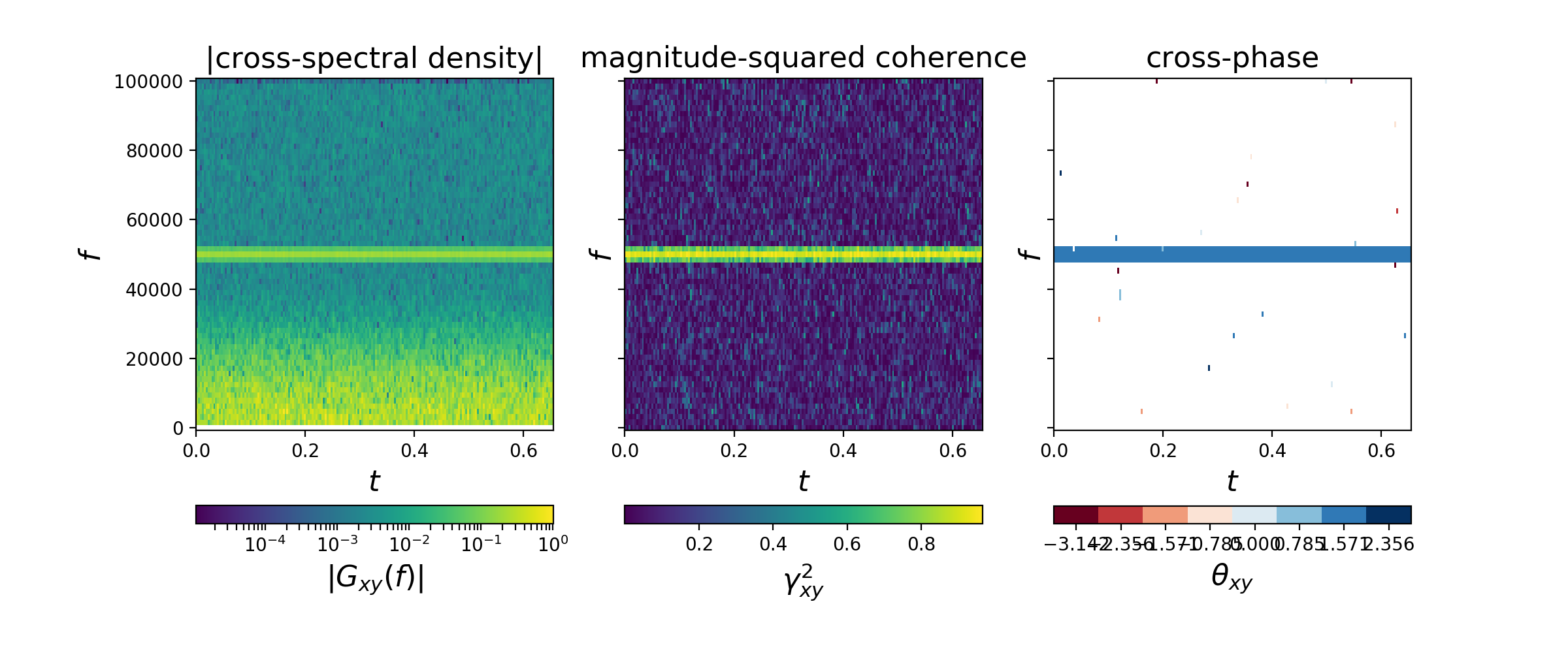
Note that the cross-phase angle (pi / 2) is correctly identified in the above spectral calculations. Further, note that the cross-phase is only plotted for points with magnitude-squared coherence exceeding a user-specified threshold.

If only one signal is available for analysis, the random_data.spectra.AutoSpectralDensity class is available for computing autospectral densities. (Of course, by definition, the coherence is unity and the phase angle zero for all frequencies and times in the autospectral density).

Spectral calculations on arrays of more than two spatially coherent signals:

If more than two measurements are available, noise in mode-number calculations can be greatly reduced by fitting the cross-phase angles of each individual measurement pair to a linear model. The random_data.array.FittedCrossPhaseArray class allows for easy fitting and visualization of cross-phase angles to obtain the corresponding mode numbers. For example, the below code spectrally analyzes an array of measurements of a 50 kHz signal in the presence of non-white noise and plots:

the coefficient of determination, R^2 (i.e. quality of fit, with larger R^2 being indicative of a better fit), as a function of frequency vs. time (left), and
the mode number as a function of frequency vs. time (right).

(Note that most of the code below is to generate representative fake signals, while the spectral computations only involve initialization of a single object. For analysis of DIII-D magnetics signals, for example, a simple package exists for fetching and organizing the magnetics data in a format that is readily compatible with random_data.array.FittedCrossPhaseArray.)

import numpy as np
import matplotlib.pyplot as plt
import random_data as rd

# =============================================================================
# Generate some fake data:
# ------------------------
# Parameters of digitized record
Fs = 200e3  # sample rate, [Fs] = samples / s
t0 = 0      # initial time, [t0] = s
T = 0.2     # (approximate) record length, [T] = s

# Measurement locations
locations = (np.pi / 180) * np.array(
    [67.5, 97.4, 127.8, 137.4, 157.6, 246.4, 277.5, 307, 312.4, 317.4, 339.8])
Nsig = len(locations)

# Generate representative random signal
tau = 8. / Fs
sig = rd.signals.RandomSignal(Fs=Fs, t0=t0, T=T, tau=tau)
Npts = len(sig.t())

# Initialize signal array
signals = np.zeros((Nsig, Npts))

# Coherent signal properties
A0 = 25.   # amplitude, [A0] = [sig1.x]
f0 = 50e3  # frequency, [f0] = Hz
n = -3     # mode number
omega0_t = 2 * np.pi * f0 * sig.t()

# Loop through measurement locations, creating corresponding
# coherent signal corrupted by noise at each point
for i in np.arange(Nsig):
    # Phase shift from mode number
    dtheta = n * (locations[i] - locations[0])

    # Coherent signal with mode-number dependence
    signals[i, :] = A0 * np.cos(omega0_t + dtheta)

    # Uncorrelated noise
    signals[i, :] += (rd.signals.RandomSignal(Fs=Fs, t0=t0, T=T, tau=tau)).x
# =============================================================================

# =============================================================================
# Perform spectral analysis:
# --------------------------
# Spectral-estimation parameters
Tens = 5e-3        # ensemble time, [Tens] = s
Nreal_per_ens = 4   # number of realizations per ensemble

A = rd.array.FittedCrossPhaseArray(
    signals, locations, Fs=sig.Fs, t0=sig.t0,
    Tens=Tens, Nreal_per_ens=Nreal_per_ens)

# Create plots
fig, axes = plt.subplots(1, 2, sharex=True, sharey=True)
A.plotR2(ax=axes[0], title='R^2')
A.plotModeNumber(ax=axes[1], title='mode number')
plt.tight_layout()
plt.show()
# =============================================================================

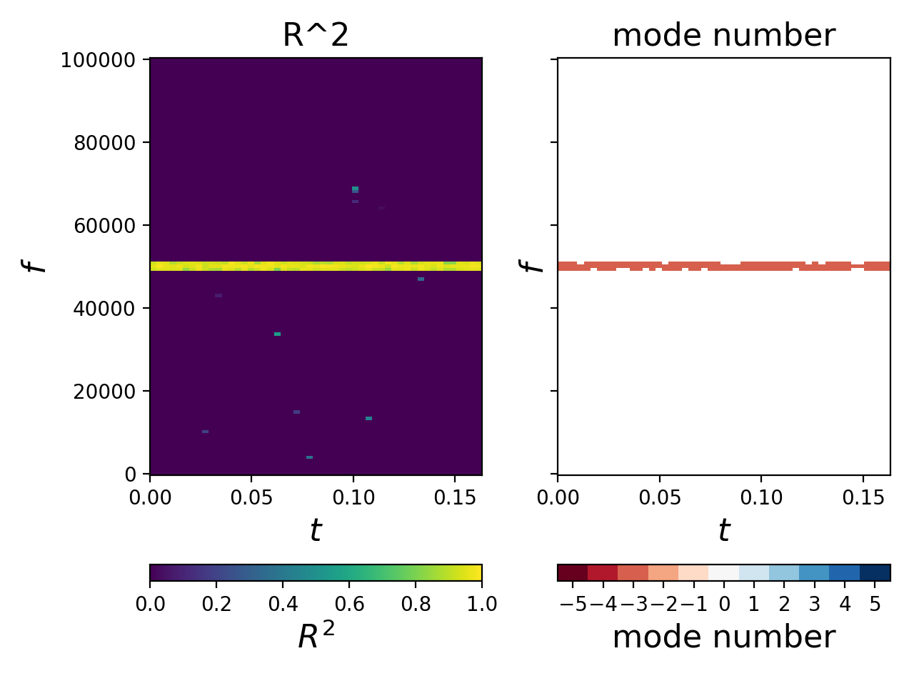
Note that the mode number (n = -3) is correctly identified in the above computations. Further, note that the mode number is only plotted for points with R^2 exceeding a user-specified threshold that can be specified on the fly.

Further, to easily examine the fit at a given frequency and time (say 50 kHz and 0.05 s), simply use:

# Using the object `A` created from running the above code
A.plotSlice('theta_xy', f=50e3, t=0.05)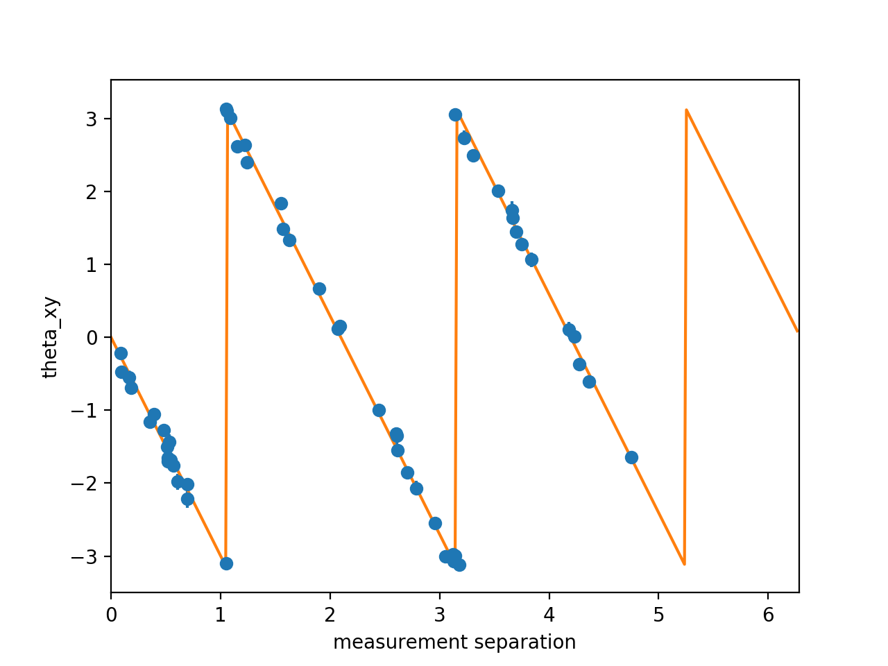

The error bars (barely visible) indicate the random error in the estimated cross-phase angle. Plotting slices of other spectral quantities ('Gxy' for cross-spectral density, 'gamma2xy' for magnitude-squared coherence) can be similarly created by substituting the appropriate string in place of 'theta_xy'.

Spectral calculations on arrays of more than two spatially broadband signals:

If more than two measurements are available and there is a broadband spatial component, a two-dimensional autospectral density S(xi, f), where xi is the spatial frequency and f is the temporal frequency, can be much more informative that the mode-number spectra above. The random_data.spectra2d.TwoDimensionalAutoSpectralDensity class allows for easy computation and visualization of S(xi, f); the random_data.spectra2d.TwoDimensionalAutoSpectralDensity class takes a complex-valued, spatial cross-correlation function as input, which can similarly be easily computed and visualized via the random_data.array.SpatialCrossCorrelation class. For example, the below code computes the two-dimensional complex-valued correlation function and the two-dimensional autospectral density of a model signal with multiple fluctuation branches.

(Note that most of the code below is to generate a model signal with multiple fluctuation branches, while the spectral computations only involve initialization of two objects, one for the correlation function and one for the two-dimensional autospectral density. For analysis of DIII-D PCI signals, for example, a package exists for fetching and organizing the PCI data in a format that is readily compatible with random_data.array.SpatialCrossCorrelation.)

import numpy as np
import matplotlib.pyplot as plt
import random_data as rd

# =============================================================================
# Signal parameters:
# ------------------
# Spatial-grid parameters
Fs_spatial = 1  # spatial sample rate, [Fs_spatial] = samples / [distance]
z0 = 0          # initial spatial sample, [z0] = 1 / [Fs_spatial]
Z = 512

# Temporal-grid parameters
Fs = 1.         # sample rate, [Fs] = samples / s
t0 = 0          # initial time, [t0] = s
T = 32768       # (approximate) temporal record length, [T] = s

# Parameters of each fluctuation branch
# (Here, we specify 4 distinct branches, each with unique characteristics)
xi0 = [0.0,   0., -0.075,   0.2]
Lz = [ 2.5,   4.,    25.,   50.]
f0 = [  0.,   0.,     0.,   0.2]
tau = [10.,  10.,    25.,  100.]
v = [  0.5, -0.5,    -4.,    0.]
S0 = [  1.,   1.,    0.1,    3.]

# Noise-floor parameters
noise_floor = 1e-5
seed = None

# Create signal object:
# ---------------------
sig = rd.signals.RandomSignal2d(
    Fs_spatial=Fs_spatial, z0=z0, Z=Z,
    Fs=Fs, t0=t0, T=T,
    xi0=xi0, Lz=Lz, f0=f0, tau=tau, v=v, S0=S0,
    noise_floor=noise_floor, seed=seed)

# Sample only a subset of spatial locations:
# ------------------------------------------
# Why? The answer is twofold:
#
# (1) The broadband signal is constructed via the inverse FFT, which
#     implicitly imposes periodicity in the spatial and temporal domains.
#     This produces a complex-valued, spatial cross-correlation function
#     that has large correlations at large spatial separations, which
#     is not typically seen in actual experimental data. Restricting
#     the spatial sampling to *at most* one half of the spatial domain
#     prevents these "unphysical" correlations.
#
# (2) In practice, sampling in time is "cheap" while sampling in space
#     is "expensive" (i.e. additional channels can require large upfront
#     capital investment). Thus, in practice, the number of channels
#     is often limited. Above, we created a broadband signal with a
#     high degree of spectral resolution, but we may not have the
#     required number of channels to reconstruct the spectrum at
#     the full resolution.
#
# The spatial sampling can be easily altered by changing the parameter
# `spatial_sampling` below.
spatial_sampling = slice(None, 32)
x = sig.x[spatial_sampling, :]
z = sig.z()[spatial_sampling]
# =============================================================================

# =============================================================================
# Complex-valued, spatial cross-correlation function:
# ---------------------------------------------------
Nreal_per_ens = 100  # number of realizations per ensemble

corr = rd.array.SpatialCrossCorrelation(
    x, z, Fs=Fs, t0=t0,
    Nreal_per_ens=Nreal_per_ens)

corr.plotNormalizedCorrelationFunction()
plt.show()

# Two-dimensional autospectral density:
# -------------------------------------
# ... via Fourier method
asd2d_fourier = rd.spectra2d.TwoDimensionalAutoSpectralDensity(
    corr, spatial_method='fourier',
    fourier_params={'window': np.hanning})

# ... via Burg method
p = 15               # AR order for Burg estimate
Nxi = 1000           # Number of points in spatial grid for Burg estimate

asd2d_burg = rd.spectra2d.TwoDimensionalAutoSpectralDensity(
    corr, spatial_method='burg',
    burg_params={'p': p, 'Nxi': Nxi})

# Compare true autospectral density to Fourier and Burg methods:
# --------------------------------------------------------------
fig, axs = plt.subplots(1, 3, figsize=(9, 4.25))
fontsize = 12
vlim = [sig._noise_floor, np.max(sig._Sxx)]

sig.plotSpectralDensity(
    ax=axs[0],
    title='true',
    fontsize=fontsize,
    vlim=vlim)
asd2d_fourier.plotSpectralDensity(
    ax=axs[1],
    title='FFT in space',
    fontsize=fontsize,
    vlim=vlim)
asd2d_burg.plotSpectralDensity(
    ax=axs[2],
    title='p = %i Burg AR in space' % p,
    fontsize=fontsize,
    vlim=vlim)

plt.tight_layout()

# Tight layout alters tick labels...
for ax in axs:
    ax.set_xticks([-0.5, -0.25, 0, 0.25, 0.5])
    ax.set_yticks([0.1, 0.2, 0.3, 0.4, 0.5])

plt.show()

# # Compare Fourier and Burg methods
# vlim = [noise_floor, np.max(sig._Sxx)]
# fig, axes = plt.subplots(1, 2, sharex=True, sharey=True, figsize=(12, 5))
# asd2d_fourier.plotSpectralDensity(ax=axes[0], title='Fourier', vlim=vlim)
# asd2d_burg.plotSpectralDensity(ax=axes[1], title='Burg', vlim=vlim)
# plt.show()
# =============================================================================

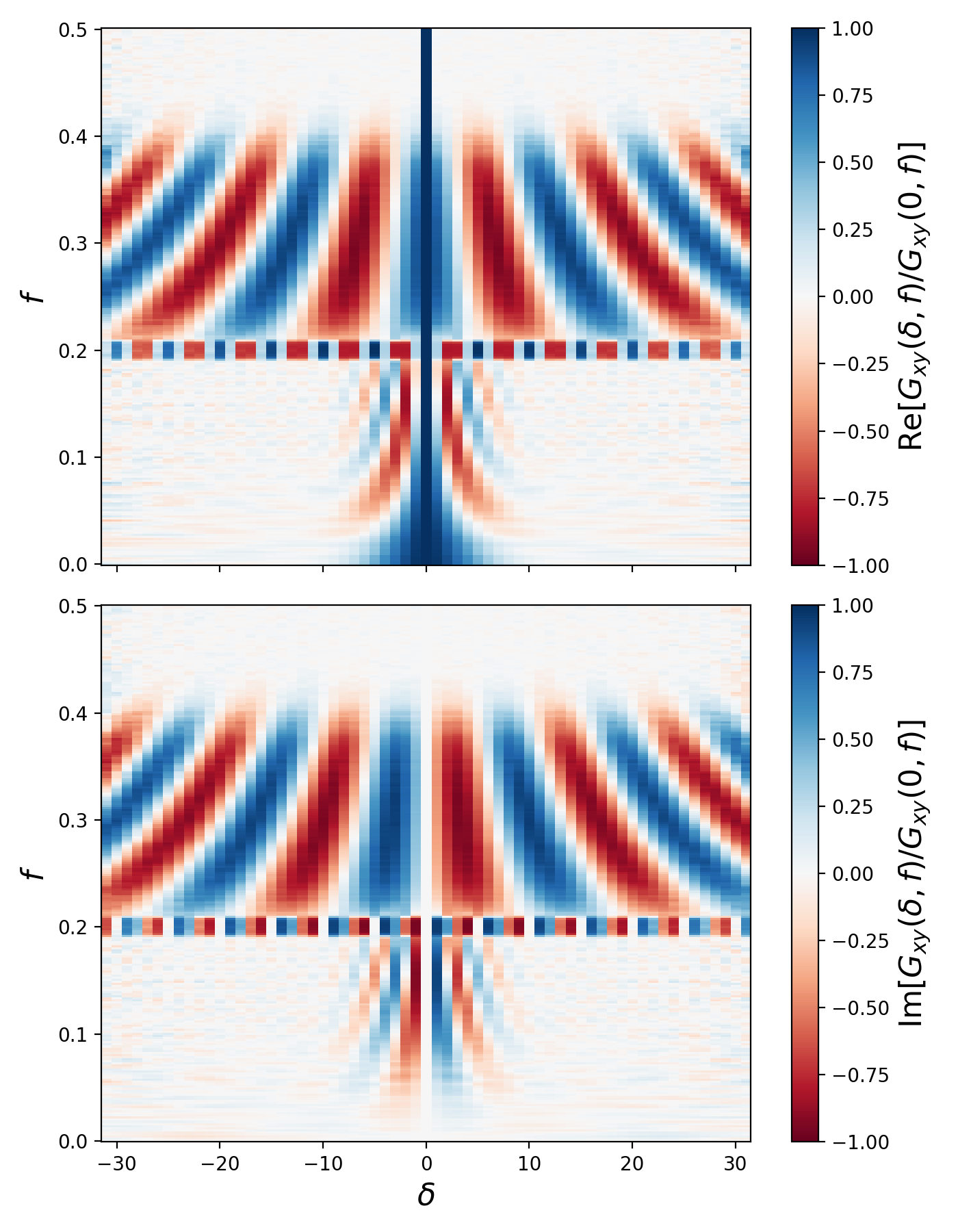
Here, contributions from both the broadband and coherent signals are visible. Note that this is a plot of the normalized complex-valued, spatial cross-correlation function. That is, at each frequency f, the correlation function Gxy(delta, f) is normalized to Gxy(0, f) (i.e. its value at zero separation (delta = 0) and frequency f). This allows for easy visualization of the correlation function's structure even if Gxy(delta, f) varies by several orders of magnitude as the frequency varies.

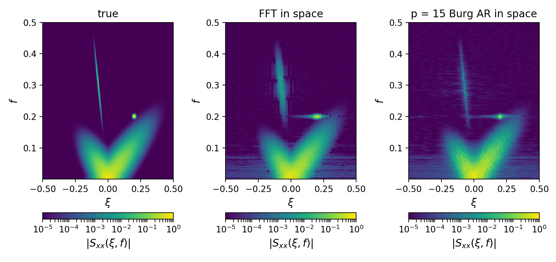
Here, in the two-dimensional autospectral density estimates, the contributions from both the broadband and coherent signals are clearly visible. Note that f is the temporal frequency and that xi is the spatial frequency (related to the usual wavenumber k via k = 2 * np.pi * xi). Further, note that the spatial spectral estimates can be estimated from the correlation function corr via a 'fourier' or 'burg' method. The Burg method can produce superior resolution particularly when the number of spatial samples are limited, but the Burg method is also subject to "pole splitting", which typically becomes more manifest as the pole order p is increased.

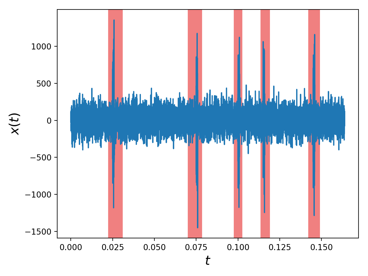
Spike identification and handling:

Spikes, whether physical or an artifact of a given measurement, may find their way into a random signal. Such spikes must be removed from the signal prior to performing spectral calculations to prevent corruption of the spectral estimates. The random_data.signals.SpikeHandler class allows for robust identification and visualization of spikes and easy removal of spike-induced contributions to the spectral estimates.

(Note that most of the code below is to generate representative fake signals, while spike identification only requires initialization of a single object and spike visualization only requires the subsequent evaluation of a single method.)

import numpy as np
import matplotlib.pyplot as plt
import random_data as rd

# =============================================================================
# Generate some fake data:
# ------------------------
# Parameters of digitized record
Fs = 200e3  # sample rate, [Fs] = samples / s
t0 = 0      # initial time, [t0] = s
T = 0.2     # (approximate) record length, [T] = s

# Generate representative random signal
f0 = 0.
tau = 4. / Fs
G0 = 1.
noise_floor=1e-5
seed = None
sig = rd.signals.RandomSignal(
    Fs=Fs, t0=t0, T=T,
    f0=f0, tau=tau, G0=G0,
    noise_floor=noise_floor, seed=seed)

# Add "spikes" to various points of signal
N = 200
spike = 3 * np.std(sig.x) * np.random.randn(N)
sig.x[5000:(5000 + N)] += spike
sig.x[15000:(15000 + N)] -= spike
sig.x[20000:(20000 + N)] += spike
sig.x[23000:(23000 + N)] -= spike
sig.x[29000:(29000 + N)] += spike
# =============================================================================

# =============================================================================
# Detect spikes:
# --------------
sigma_mult = 5      # detect spikes that at 5x the RMS of `sig.x`
debounce_dt = 5e-3  # distinct spikes must be at least 5 ms apart

SH = rd.signals.SpikeHandler(
    sig.x, Fs=sig.Fs, t0=sig.t0,
    sigma_mult=sigma_mult, debounce_dt=debounce_dt)

# Plot original signal, highlighting spikes:
# ------------------------------------------
window_fraction = [0.1, 0.9]
SH.plotTraceWithSpikeColor(sig.x, sig.t(), window_fraction=window_fraction)
plt.tight_layout()
plt.show()
# =============================================================================

The effects of including vs. excluding the spikes from the spectral computations can be easily evaluated:

# Spectral calculations:
# ----------------------
# Spectral-estimation parameters
Tens = 1e-3         # ensemble time, [Tens] = s; *LESS* than spike spacing!!!
Nreal_per_ens = 1   # will perform averaging later, after spike removal

asd = rd.spectra.AutoSpectralDensity(
    sig.x, Fs=sig.Fs, t0=sig.t0,
    Tens=Tens, Nreal_per_ens=Nreal_per_ens)

# Average over all contributions, including spikes
Gxx_raw = np.mean(asd.Gxx, axis=-1)

# Average only over `window_fraction` of spike-free windows
ind = SH.getSpikeFreeTimeIndices(asd.t, window_fraction=window_fraction)
Gxx_no_spikes = np.mean(asd.Gxx[:, ind], axis=-1)

# Plot difference between raw and spike-free spectra:
# ---------------------------------------------------
fontsize = 16

plt.figure()
plt.loglog(asd.f, Gxx_raw, 'r')
plt.loglog(asd.f, Gxx_no_spikes, 'b')
plt.xlabel(r'$f$', fontsize=fontsize)
plt.ylabel(r'$G_{xx}(f)$', fontsize=fontsize)
plt.legend(['raw (w/ spikes)', 'w/o spikes'],
           loc='lower left', fontsize=fontsize)
plt.show()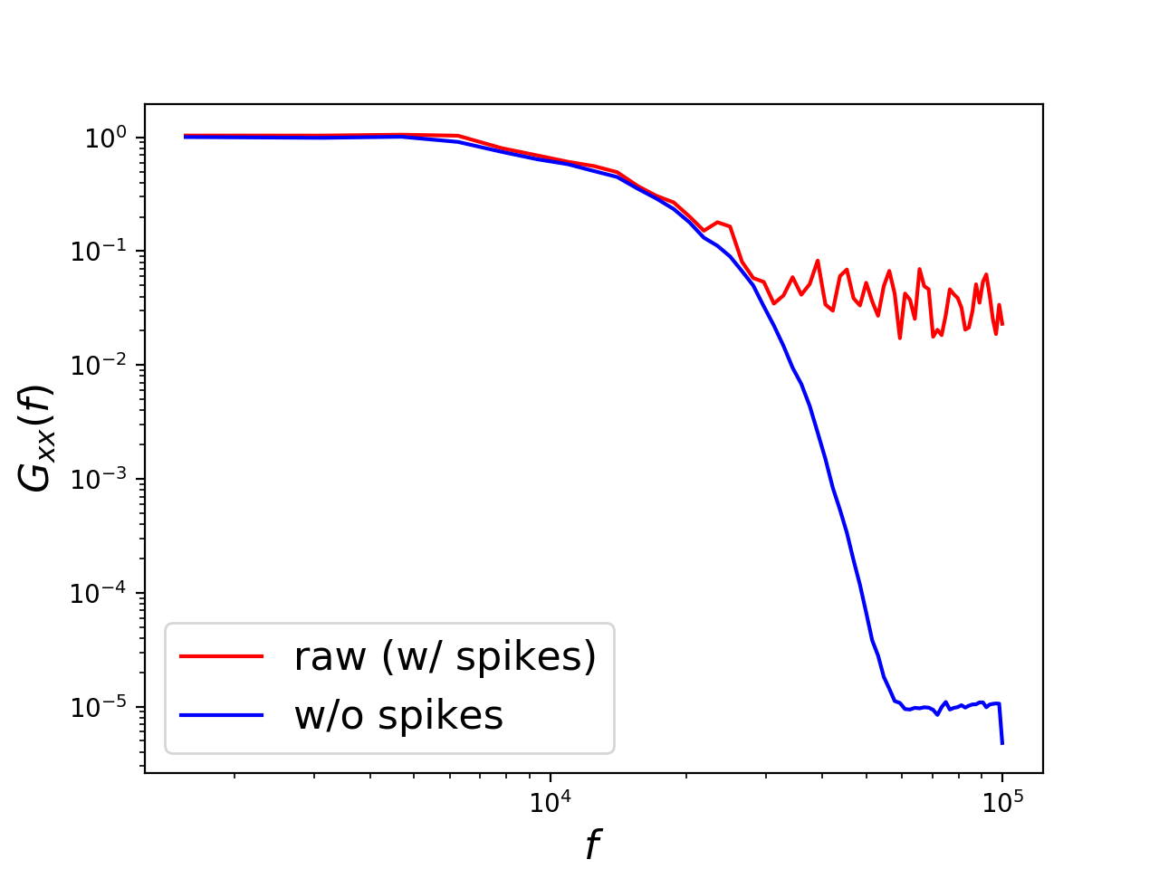

Trigger offset: estimation and compensation

Accurately estimating spectral quantities of a given random process from a collection of digital records requires (among other things) that the true, physical timebase of the process is well-represented by the nominal timebase of the digital record. If two records x1 and x2 have the same nominal time base but, for example, digitization of record x2 actually begins a finite time tau later than the digitization of record x1, then naively computed spectral estimates will be biased away from their true, physical values.

The random_data.signals.TriggerOffset class allows for easy estimation of such trigger offsets, as demonstrated below. (Note that most of the code below is required to generate representative fake signals and to visualize the data, while estimating the trigger only requires initialization of a single object; subsequent compensation of the trigger offset only requires calling a single function).

import numpy as np
import matplotlib.pyplot as plt
import random_data as rd

# =============================================================================
# Generate some fake data:
# ------------------------
# Nominal temporal-grid parameters
Fs = 1.                         # sample rate, [Fs] = arbitrary units
t0 = 0                          # nominal trigger time, [t0] = s
T = 1e5                         # (approximate) record length, [T] = s

# Discrepancy `tau` between timebase of digital record 1 and
# timebase of digital record 2. Note that, as defined here,
# `tau` is *not* an integer of the sample spacing; that is,
# the trigger-offset estimation and compensation works for
# arbitrary `tau`.
tau = 0.5 / Fs                  # [tau] = s, nonzero

# Spectral parameters of broadband signal common to digital records 1 & 2
f0_broad = 0.
tau_broad = 2. / Fs  # correlation time
G0 = 1.
seed = None

sig = rd.signals.RandomSignal(
    Fs=Fs, t0=t0, T=T,
    f0=f0_broad, tau=tau_broad, G0=G0,
    noise_floor=0., seed=seed)
N = len(sig.x)
t = sig.t()

# Generate two digital records that are identical *except* for
# timebase offset `tau`. Note that `x1[0]` physically occurs at
# time `t[0]`, while `x2[0]` physically occurs at time `t[0] + tau`.
x1 = sig.x.copy()
x2 = rd.signals.sampling.circular_resample(sig.x, Fs, tau)

# Add uncorrelated noise
Gnn = 1e-6                      # [Gnn] = [signal]^2 / [Fs]
noise_power =  Gnn * (0.5 * Fs)
noise_amplitude = np.sqrt(noise_power)
x1 += (noise_amplitude * np.random.randn(N))
x2 += (noise_amplitude * np.random.randn(N))
# =============================================================================

# =============================================================================
# Estimate trigger offset and compensate:
# ---------------------------------------
# Spectral-estimation parameters
Tens = t[-1] - t[0]             # [Tens] = [s]; full record is 1 ensemeble
Nreal_per_ens = 1000            # [Nreal_per_ens] = unitless
gamma2xy_max = 0.95             # [gamma2xy_max] = unitless

# Estimate trigger offset
trig = rd.signals.TriggerOffset(
    np.array([x1, x2]),
    gamma2xy_max=gamma2xy_max,
    Fs=Fs,
    Nreal_per_ens=Nreal_per_ens)

print '\ntrue trigger offset: %f' % tau
print 'estimated trigger offset: %f' % trig.tau

# Now, use estimated value to compensate for trigger offset
x2_corrected = rd.signals.sampling.circular_resample(x2, Fs, -trig.tau)
# =============================================================================

# =============================================================================
# Examine cross phase between for uncorrected and corrected records:
# ------------------------------------------------------------------
csd_uncorr = rd.spectra.CrossSpectralDensity(
    x1, x2, Fs=Fs, t0=t0,
    Tens=Tens, Nreal_per_ens=Nreal_per_ens)
csd_corr = rd.spectra.CrossSpectralDensity(
    x1, x2_corrected, Fs=Fs, t0=t0,
    Tens=Tens, Nreal_per_ens=Nreal_per_ens)

plt.figure()
plt.axhline(0, c='k', label='expected')
plt.plot(csd_uncorr.f, np.squeeze(csd_uncorr.theta_xy), label='uncorrected')
plt.plot(csd_corr.f, np.squeeze(csd_corr.theta_xy), label='corrected')
plt.xlabel('f [Fs]')
plt.ylabel('cross phase [rad]')
plt.legend(loc='best')
plt.show()
# =============================================================================

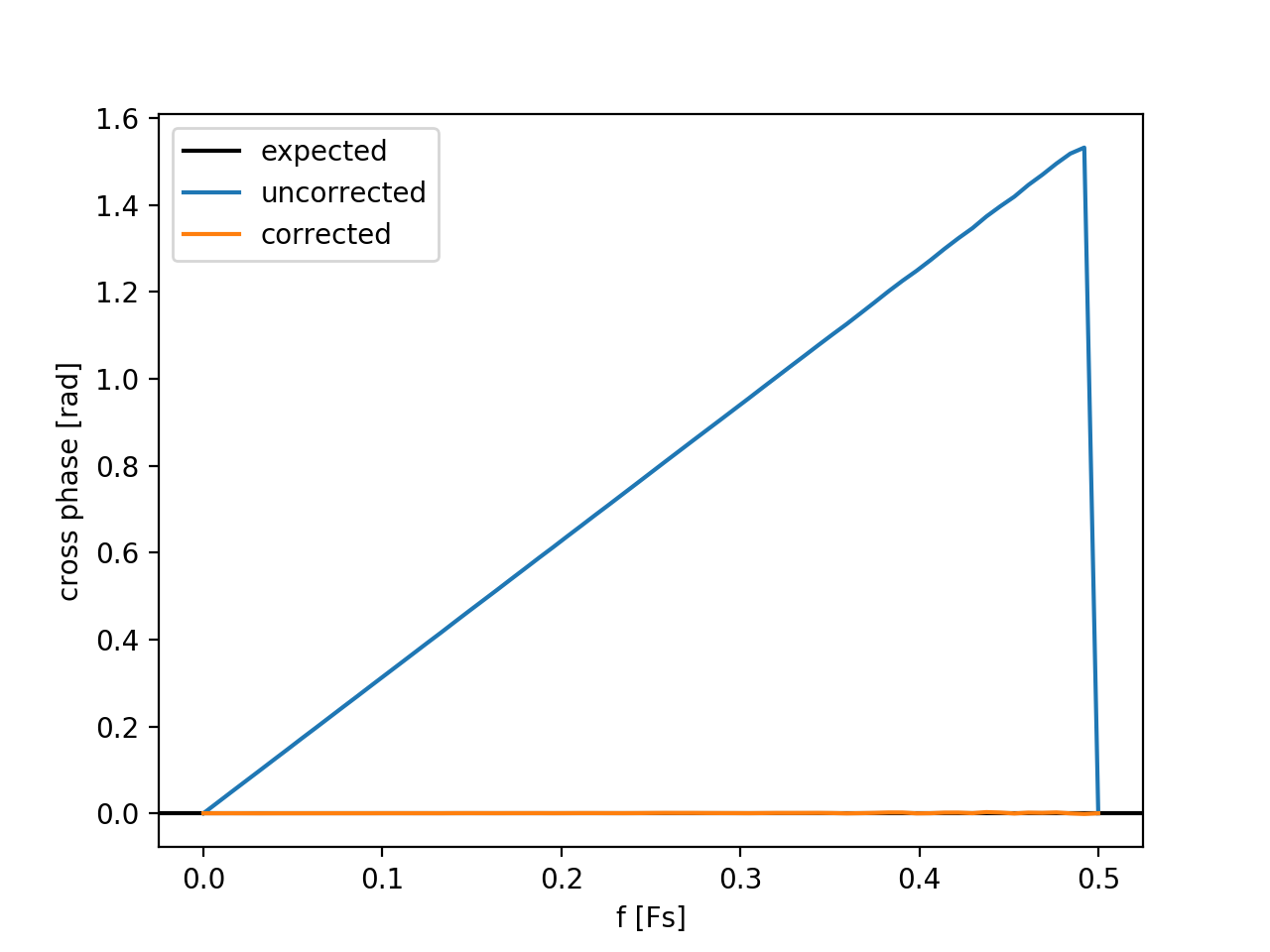
Note that cross phase computed after compensating for the trigger offset is in agreement with expectations. The large fluctuations in the computed cross phase at high frequencies is attributable to the low signal-to-noise ratio (SNR) at these frequencies; the trigger-offset algorithm is weighted such that points with low SNR minimally contribute to the offset estimate.

Name		Name	Last commit message	Last commit date
Latest commit History 330 Commits
figs		figs
random_data		random_data
tests		tests
.gitignore		.gitignore
LICENSE		LICENSE
README.md		README.md
setup.py		setup.py

Provide feedback

Saved searches

Use saved searches to filter your results more quickly

figs

figs

random_data

random_data

tests

tests

.gitignore

.gitignore

LICENSE

LICENSE

README.md

README.md

setup.py

setup.py

Repository files navigation

Background:

Installation:

... on GA's Iris cluster:

... elsewhere:

Use:

Spectral calculations on two signals:

Spectral calculations on arrays of more than two spatially coherent signals:

Spectral calculations on arrays of more than two spatially broadband signals:

Spike identification and handling:

Trigger offset: estimation and compensation

About

Releases

Packages

Languages

License

emd/random_data

Folders and files

Latest commit

History

Repository files navigation

Background:

Installation:

... on GA's Iris cluster:

... elsewhere:

Use:

Spectral calculations on two signals:

Spectral calculations on arrays of more than two spatially coherent signals:

Spectral calculations on arrays of more than two spatially broadband signals:

Spike identification and handling:

Trigger offset: estimation and compensation

About

Resources

License

Stars

Watchers

Forks

Languages