There are numerous models modelled as graphs indicating the dependencies between different modules in requirements engineering. The i* framework[1] proposes an agent-oriented approach to requirements engineering centering on the intentional characteristics of the agent. Agents attribute intentional properties (such as goals, beliefs, abilities, commitments) to each other and reason about strategic relationships. Dependencies between agents give rise to opportunities as well as vulnerabilities. Networks of dependencies are analyzed using a qualitative reasoning approach. Agents consider alternative configurations of dependencies to assess their strategic positioning in a social context. The framework is used in contexts in which there are multiple parties (or autonomous units) with strategic interests which may be reinforcing or conflicting in relation to each other. Examples of such contexts include: business process redesign, business redesign, information systems requirements engineering, analyzing the social embedding of information technology, and the design of agent-based software systems. The framework consists of nodes and edges with Tasks and Resources representing input nodes, while Goals and SoftGoals representing output nodes. Edges are used to propogate values from one node to another. Edges are of four types
- Dependency : Parent depends on child. ie If the child is satisfied, then the parent is also satisfied
- Contribution : Quantitates softgoals. This edge can be of 4 types: Make, Help, Hurt and Break.
- Decomposition : Represents logical AND edges.
- Means-Ends : Represents logical OR edges.
The figure below highlights the model with an example
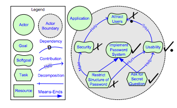
In the above figure "Restrict Structure of Password" and "Ask for Secret Question" are identified as unsatisfied and satisfied respectively. These values are propagated through the edges to compute the value of each node. The satisifability of each node is highlighted on it as the values are propogated.
Models are described in the following formats
- Smaller Models in Py* graph notation. Here
- Larger Models in Py* graph notation. Here
- Larger models in json notation. Here
- Larger models in graphviz notation. Here
- .itarml and .ood (No Parser exists)
Py* is developed in python where each node/edge is represented as a python class. The class hierachy with each base class followed by their child classes is as follows
Component
|.. Node
|.. |.. Task
|.. |.. Resource
|.. |.. Goal
|.. |.. Softgoal
|.. Edge
|.. |.. Dependency
|.. |.. Decomposition
|.. |.. |.. AND
|.. |.. |.. OR
|.. |.. Contribution
|.. |.. |.. Make
|.. |.. |.. Help
|.. |.. |.. Hurt
|.. |.. |.. Break
The graph is evaluated as follows:
- A node is selected at random from the graph.
- The incoming edges of the node are identified and all the child nodes are recursively evaluated.
- Two kinds of conflicts can arise while evaluating the nodes
- The incoming edges can be conflicting. For example, one incoming edge can be help, while the other can be hurt. In such cases a random value(satisfied or unsatisfied) is assigned to the node.
- A loop can exist. i.e While propagating through the nodes, we notice that the same node is visited again. In such cases too, a random value is assigned to the node.
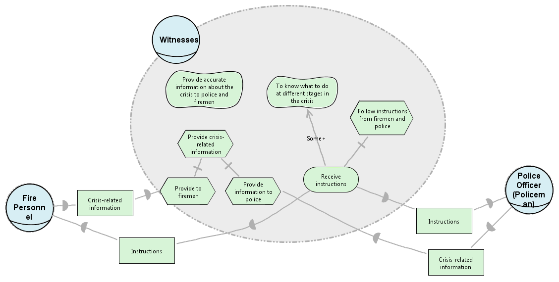
A sample model shown above is represented as follows
from template import *

N = Many()
# Nodes
n1 = N + SoftGoal(name = "Provide accurate Information", container="Witnesses")
n2 = N + SoftGoal(name = "To know what to do", container="Witnesses")
n3 = N + Task(name = "Follow instructions from firemen", container="Witnesses")
n4 = N + Task(name = "Provide crisis related info", container="Witnesses")
n5 = N + Task(name = "Provide to fireman", container="Witnesses")
n6 = N + Task(name = "Provide info to police", container="Witnesses")
n7 = N + HardGoal(name = "Receive instructions", container="Witnesses")
n8 = N + Resource(name = "Crisis-related information", container="Fire")
n9 = N + Resource(name = "Instructions", container="Fire")
n10 = N + Resource(name = "Instructions", container="Police")
n11 = N + Task(name = "Crisis-related information", container="Police")

E = Many()
#Edges
e1 = E + SomePlus(source = n7,target = n2)
e2 = E + Or(source = n7,target = n3)
e3 = E + And(source = n5,target = n4)
e4 = E + And(source = n6,target = n4)
e5 = E + Dep(source = n5,target = n8)
e6 = E + Dep(source = n9,target = n7)
e7 = E + Dep(source = n10,target = n7)
e8 = E + Dep(source = n6,target = n11)

graph = Graph(name="bCMS_SR_Witness", nodes=N.all, edges=E.all)Optimization is performed using differential evolution

We first rank the decisions usingKruns of the differential evolution algorithm. The Kruns aredivided based on Non Dominated Sorting into
- best: Points associated with the top BEST% points.
- rest: Points that are not included in best.
The algorithm then computes the probability that a decision is found in best using Bayes Theorem. Informally, the theorem says that ** posterior = prior * likelihood ** More formally:
P(H|E)=P(E|H) * P(H) / P(E)
i.e using evidence E and a prior probability P(H) for hypothesis H ∈ {best, rest}. The theorem calculates the posterior probabilityP(H|E). When applying the theorem, likelihoods are computed from observed frequencies, then normalized to create probabilities (this normalization cancels outP(E)in Eq. 4.2, so it need not becomputed). For example after K=10,000 runs divide into 1,000 lowest 10% best solutions and 9,000 rest, the decision X=x might appear 10 times in the best solutions, butonly 5 times in the rest. This can be formulated as follows:
E = (X=x)
P(best) = 1000/10000 = 0.1
P(rest) = 9000/10000 = 0.9
freq(E|best) = 10/1000 = 0.01
freq(E|rest) = 5/9000 = 0.00056
like(best|E) = freq(E|best) * P(best) = 0.001
like(rest|E) = freq(E|rest) * P(rest) = 0.00050
P(best|E) = like(best|E) / (like(best|E) + like(rest|E))
P(best|E) * support(best|E) = like(best|E)^2 / (like(best|E) + like(rest|E))
- SAMPLE: To sample the decisions form the models, STAR1 runs the Differential Evolution algorithm K1times.
- CLASSIFY: The outcomes of the runs are then ranked into those seen in BEST% as best and the remaining into rest.
- RANK: The decisions along with their optimal values are then ranked using Non Dominated Sorting in the decreasing order by their probability * support of appearing in thebest outcomes.
- PRUNE: The algorithm then runs K2 experiments with the models where the top ranked decisions between 1...X are pre-set to their optimal value as computed on the previous step. The remaining decisions are assigned random values. This step is crucial as we identify the significance of each decision and its contribution towards the satisfaction of the model's objectives.
- REPORT: The algorithm finally plots the median and Inter-Quartile Range(IQR) for each ofthe 1 . . .X decisions which the analyst can use to identify the significance of the decisions.
1 Setup the dependencies using pip
pip install -r requirements.txt
2 To run steps for a model
- Preset models in runner.sh
- Set the date and folder name
- Run the following command
sh runner.sh
3 The output will be saved in weekly-reports/<date>/<folder-name>/<model_name>.md
4 You would need a markdown previewer for viewing the model results.