
Python package to determine the mixing behaviour of Markov chains. Markov chains are represented by their transition matrices, using scipy sparse matrices. The mixing behaviour is determined by explicitly multiplying initial distributions with the transition matrix (many times).
The package supports general Markov chains with the class MarkovChain. There is direct support for the networkx graph package (for random walks on graphs). Whereas the focus so far is on total-variation mixing, the package can be used with other notions of distance. Running on common hardware, it is feasible to have around 100.000 states (depending on the mixing time). If you have any comments or suggestions, please file an issue or write an email to sbordt at posteo.de.
And now some examples!
import markovmixing as mkm
import networkx as nx
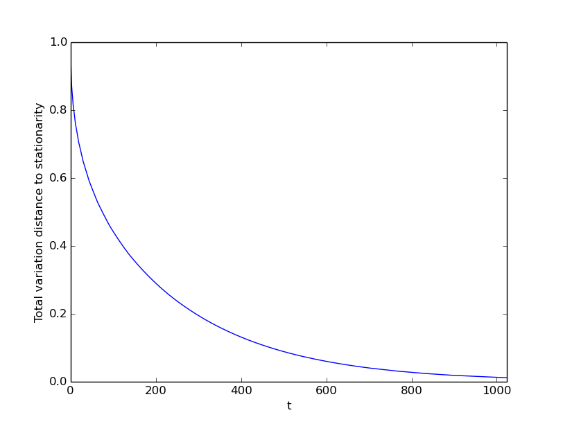
# create a networkx graph
G = nx.cycle_graph(50)
# create a MarkovChain that is lazy simple random walk on the graph
mc = mkm.nx_graph_lazy_srw(G)
# add a random delta distribution as initial distribution
mc.add_random_delta_distributions(1)
# plot the total variation mixing
mc.plot_tv_mixing(y_tol=0.01, threshold=0.01)
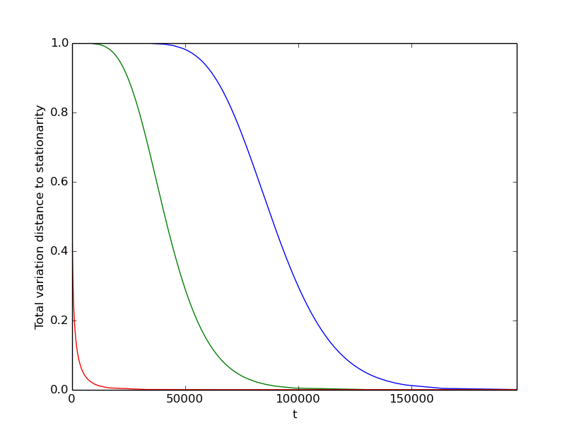
# create the transition matrix
P = mkm.line_lazy_transition_matrix(1000, p=0.51)

# create the MarkovChain with the given transition matrix
mc = mkm.MarkovChain(P)

# add some initial distributions
for i in [0,500,999]:
    mc.add_distributions(mkm.delta_distribution(1000,x=i))

# plot the total variation mixing
mc.plot_tv_mixing(y_tol=0.01, threshold=1e-5)
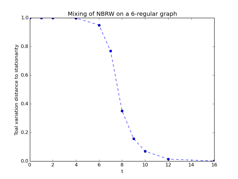
This example does not make use of plot_tv_mixing and shows the usage of some intermediate methods.
import matplotlib.pyplot as plt

# load a 6-regular graph with 50.000 nodes from file
G_6_regular = nx.read_sparse6('6_regular.s6')

# get the adjacency matrix
A = nx.to_scipy_sparse_matrix(G_6_regular)

# transition matrix for NBRW on the graph from the adjacency matrix
P = mkm.graph_nbrw_transition_matrix(A)

# Markov chain with the transition marix
mc = mkm.MarkovChain(P)

# the stationary distribution is uniform
mc.set_stationary(mkm.uniform_distribution(mc.get_n()))

# add a random starting position to the Markov chain
mc.add_distributions(mkm.random_delta_distributions(mc.get_n(),1))

# determine the mixing in total variation
mc.compute_tv_mixing()

# plot the mixing
(x,tv) = mc.distribution_tv_mixing(0)
plt.plot(x, tv)
plt.xlabel("t")
plt.ylabel("Distance to stationary distribution in total variation")
plt.show()
A Markov chain is constructed from a transition matrix.
import markovmixing as mkm
import numpy as np

P = mkm.circle_transition_matrix(5)
mc = mkm.MarkovChain(P)
Initial distributions are refered to as 'distributions', and can be added as follows.
mc.add_distributions(np.array([0,0,0,0.5,0.5]))
mc.add_random_delta_distributions(2)
Set the stationary distribution (recommended). If unknown, the package will try to determine the stationary distribution, but this is only experimental at the moment!
mc.set_stationary(np.ones(5)/5)
The purpose of this package is to determine the mixing behavior. Each initial distribution is iterated until it is sufficiently close to stationarity.
mc.iterate_all_distributions_to_stationarity()
Iterating distributions produces 'iterations'.
print mc.get_iteration_times(1)
[0, 1, 2, 4, 8]

print mc.get_iterations(1)
{0: array([ 1.,  0.,  0.,  0.,  0.]), 1: array([ 0.5 ,  0.25,  0.  ,  0.  ,  0.25]), 2: array([ 0.375 ,  0.25  ,  0.0625,  0.0625,  0.25  ]), 4: array([ 0.2734375 ,  0.22265625,  0.140625  ,  0.140625  ,  0.22265625]), 8: array([ 0.21347046,  0.2041626 ,  0.18910217,  0.18910217,  0.2041626 ])}
Given these iterations (i.e. evolved initial distributions), mixing can be computed. For total-variation distance, there is a utility method.
(t,tv) = mc.distribution_tv_mixing(1)

print t
[0, 1, 2, 4, 8]

print tv
[0.80000000000000004, 0.40000000000000002, 0.27500000000000002, 0.11874999999999999, 0.021795654296874994]
One can use
plot_tv_mixing(indices=None,y_tol=0.1,threshold=0.05,text=True)
which automatically iterates the respective distributions to stationarity and creates a plot, as in the above examples.
A summary of the chain is obtained in the following way.
mc.print_info()

This is a Markov chain with n=5. The transition matrix is:
  (0, 0)    0.5
  (0, 1)    0.25
  (0, 4)    0.25
  (1, 0)    0.25
  (1, 1)    0.5
  (1, 2)    0.25
  (2, 1)    0.25
  (2, 2)    0.5
  (2, 3)    0.25
  (3, 2)    0.25
  (3, 3)    0.5
  (3, 4)    0.25
  (4, 0)    0.25
  (4, 3)    0.25
  (4, 4)    0.5
The stationary distribution is:
[ 0.2  0.2  0.2  0.2  0.2]
The Markov chain has 3 distributions with iterations saved at the following timesteps:
[0, 1, 2, 4, 8]
[0, 1, 2, 4, 8]
[0, 1, 2, 4, 8]
The distributions:
[ 0.   0.   0.   0.5  0.5]
[ 0.  1.  0.  0.  0.]
[ 0.  0.  0.  1.  0.]
The latest iterations are:
[ 0.19663239  0.18910217  0.19663239  0.20881653  0.20881653]
[ 0.2041626   0.21347046  0.2041626   0.18910217  0.18910217]
[ 0.18910217  0.18910217  0.2041626   0.21347046  0.2041626 ]
These methods create transition matrices.
graph_srw_transition_matrix(A)
graph_nbrw_transition_matrix(A)
line_lazy_transition_matrix(n, p = 0.5)
circle_transition_matrix(n, p = 0.5, lazy = True)
hypercube_transition_matrix(n, lazy = True)
To create a MarkovChain from a networkx graph, use one of the following.
nx_graph_srw(G)
nx_graph_lazy_srw(G)
nx_graph_nbrw(G)
As always, we have some utility methods :-)
is_transition_matrix(P)
lazy(P)
is_distribution(mu,n=None)
total_variation(mu,nu)
delta_distribution(n,x=0)
random_delta_distributions(n,k=1)
uniform_distribution(n)
graph_srw_stationary_distribution(A)