The python scripts here utilize 4 python packages all available through PYPI:
- Numpy
- Scipy
- Matplotlib
- Scikit-neuralnetwork
These can all be installed through the pip command in the terminal
> pip install numpy scipy matplotlib scikit-neuralnetwork
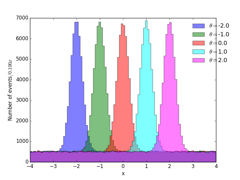
- Number of data points per signal/background: 50,000
- Signal: Gaussians at mu=-2,-1,0,1,2
- Background: Flat
- Bins: 25
- Bin Width: 0.4
Each gaussian (i.e. mu=-2, -1, 0, 1, 2) is trained with a seperate NN and then prediction outputs are plotted vs input values between [-5, 5].
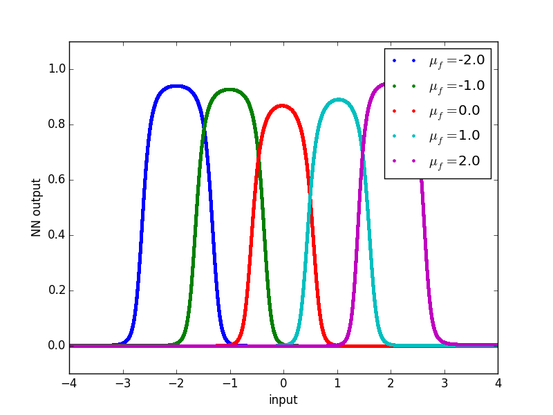
A NN is trained for gaussians at mu=-2, -1, 0, 1, 2 and predictions are made at mu=-1.5, -1, -0.5, 0, 0.5, 1, 1.5. Thus, predictions at half-odd integer values (i.e. mu=-1.5, -0.5, 0.5, 1.5) are interpolations based on training at integer values.

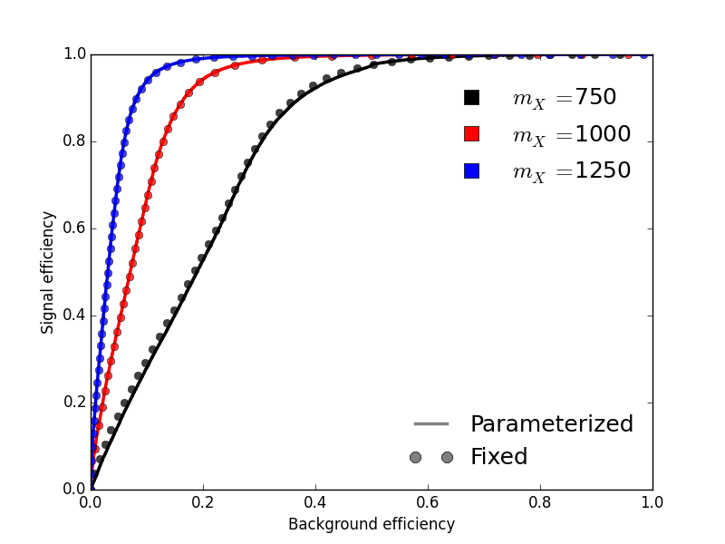
ROC curves and AUC values for the same set of predictions made in the parameterized training set (i.e. training at mu=-2, -1, 0, 1, 2 with predictions at mu=-1.5, -1, -0.5, 0, 0.5, 1, 1.5)
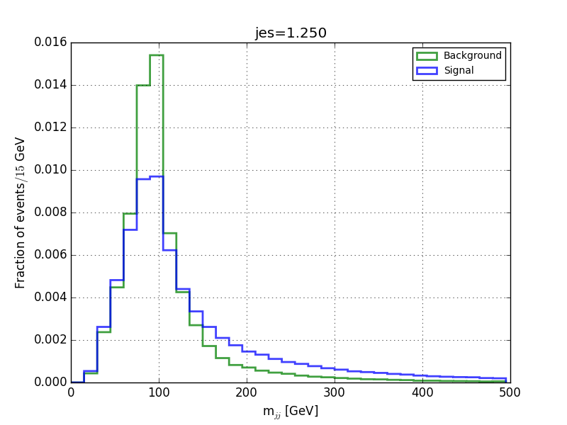
- Signal at mx = 500 GeV, 750, 1000, 1250, 1500
- Bin Width: 50 GeV
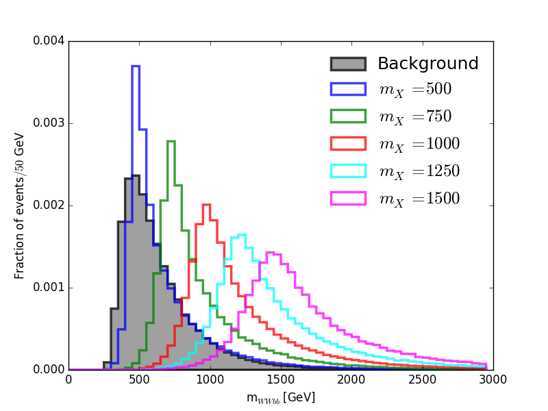
A seperate NN is trained to seperate signal and background at each of the 5 fixed mx values (mx = 500, 750, 1000, 1250, 1500) and plotted (plot lines). Next, a seperate NN is trained with for all signals and backgrounds but each time excluding one of the mx values so that this mx value can be interpolated from neighboring signals (circle markers). For example, the NN excluding mx=500 GeV (i.e. trained with mx=750 GeV, 1000, 1250, 1500) is used to predict the outputs for a signal at mx=500 GeV. Similarly, the NN trained at mx=500 GeV, 1000, 1250, 1500 (i.e. excluding mx=750 GeV) is used to predict the outputs for a signal at mx=750 GeV.

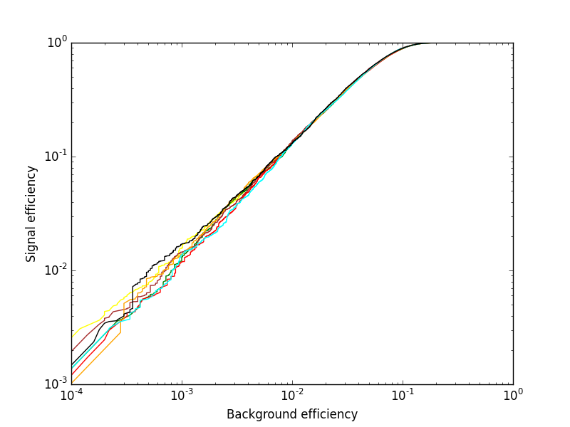
ROC curves and AUC values for the fixed and parameterized training performed in the previous section.
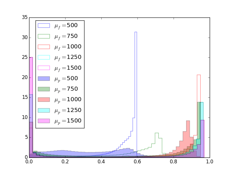
NN output for the fixed and parameterized training in the previous section is plotted as a histogram to check the way in which output is parsed between signal (1) and background (0) scores.
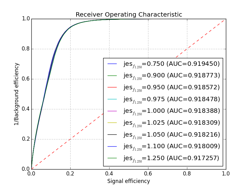
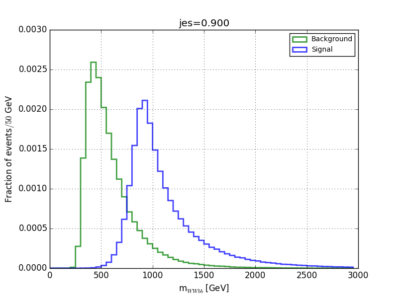
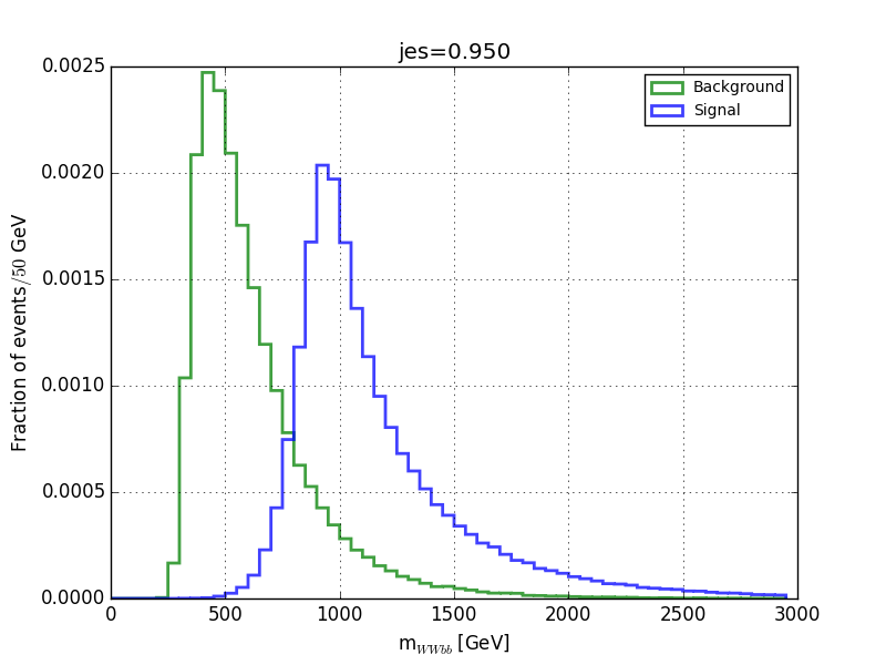
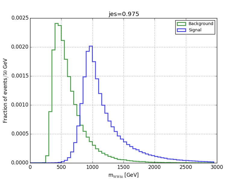
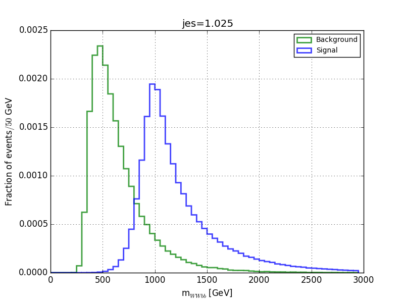
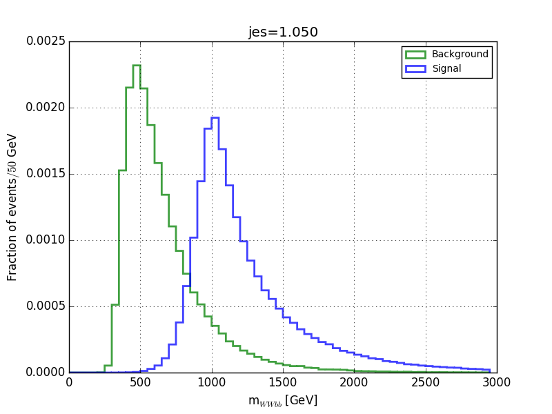
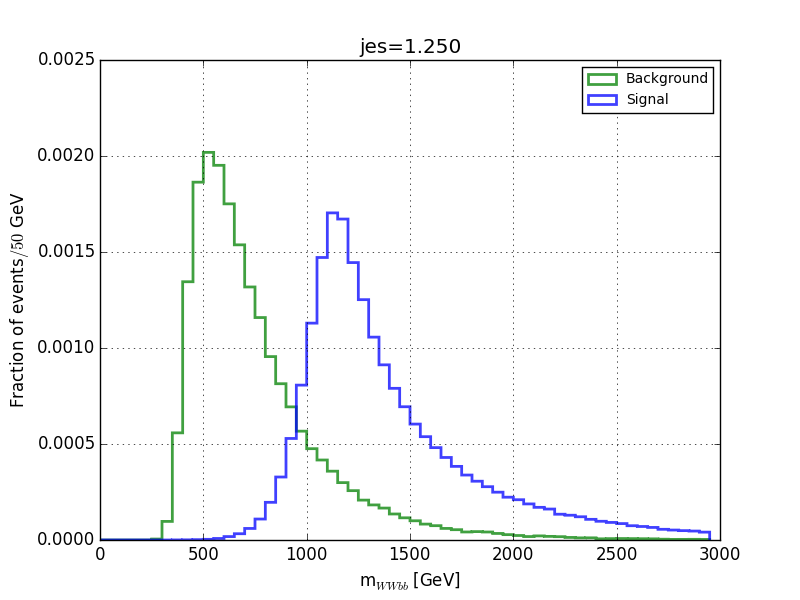
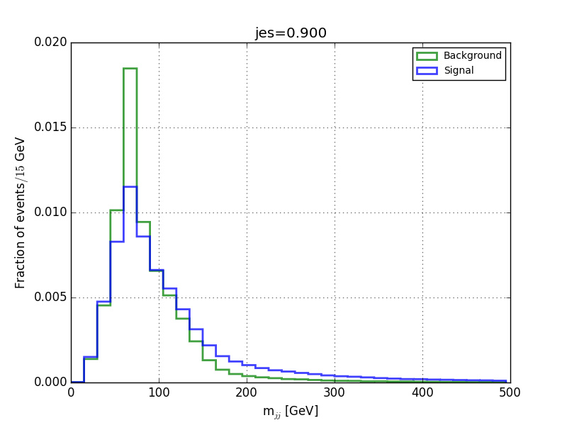
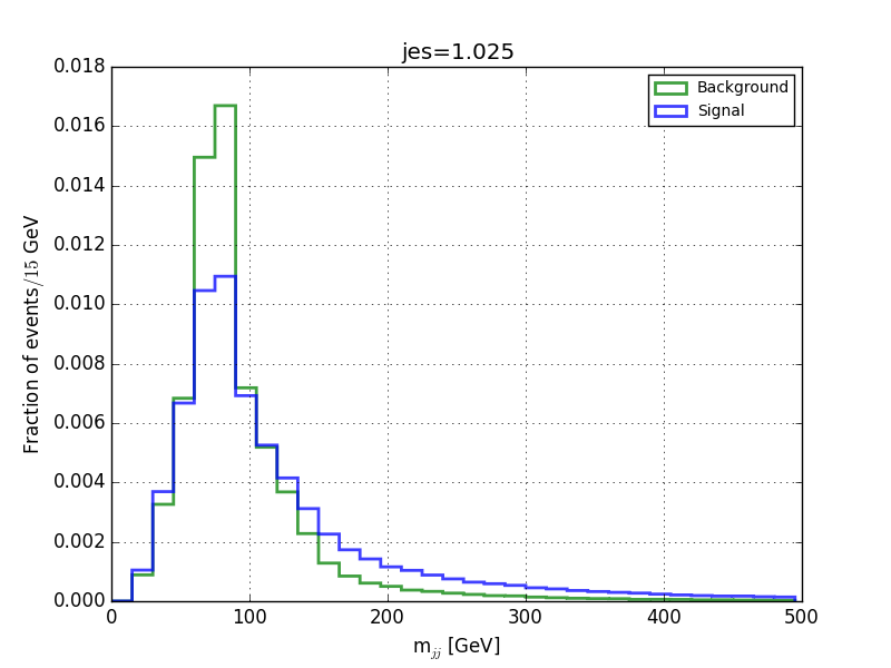
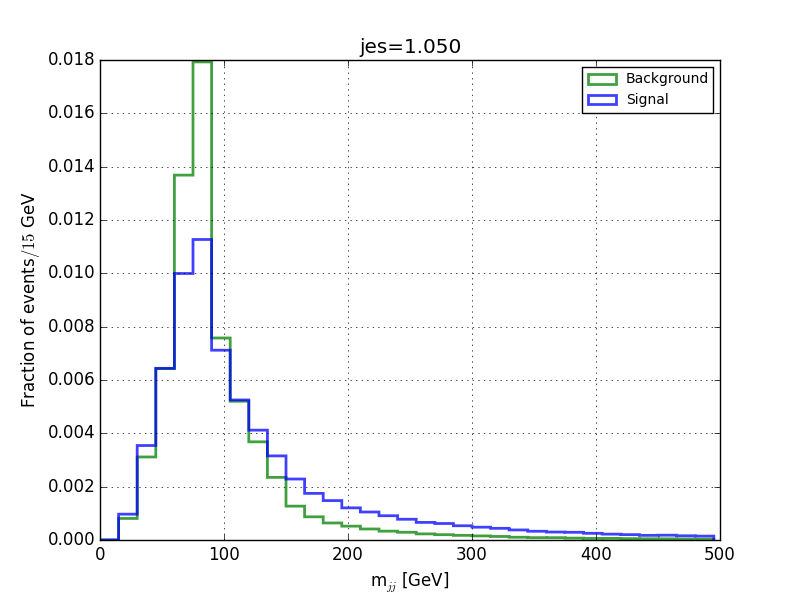
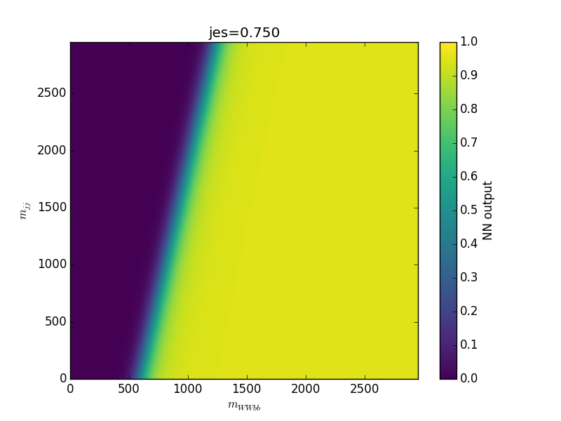
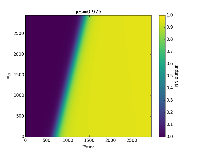
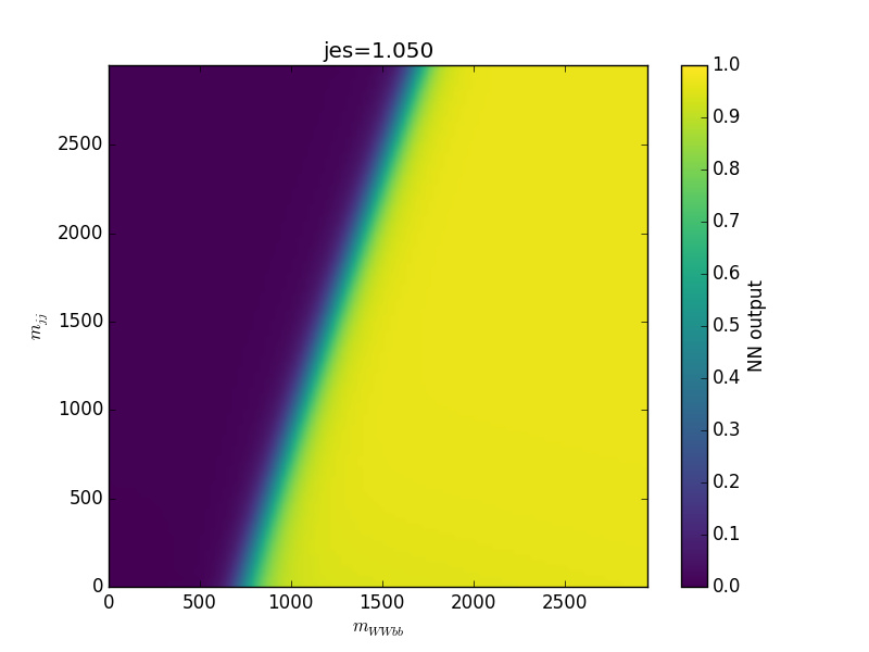
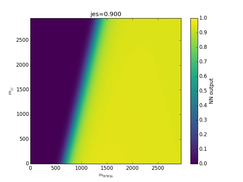
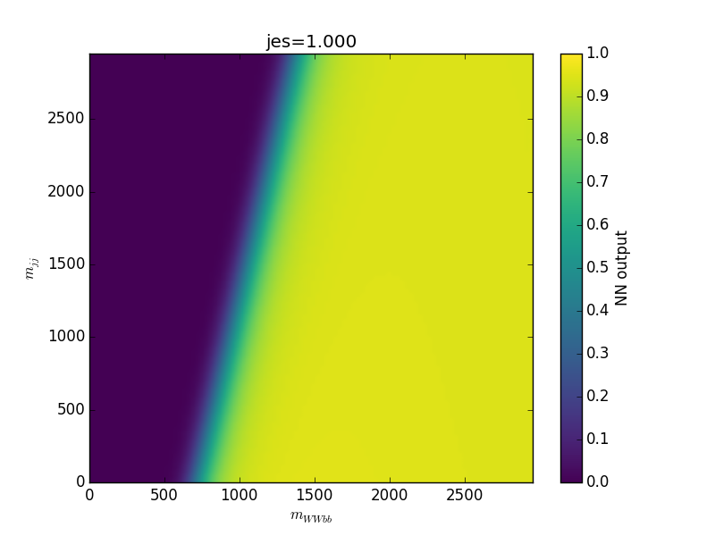
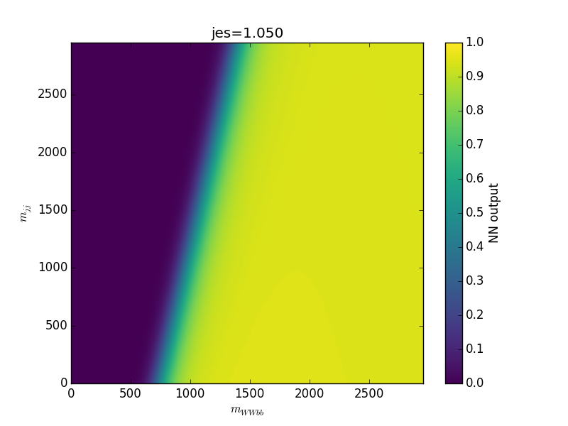
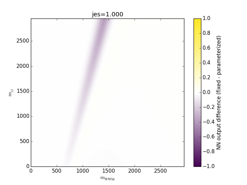
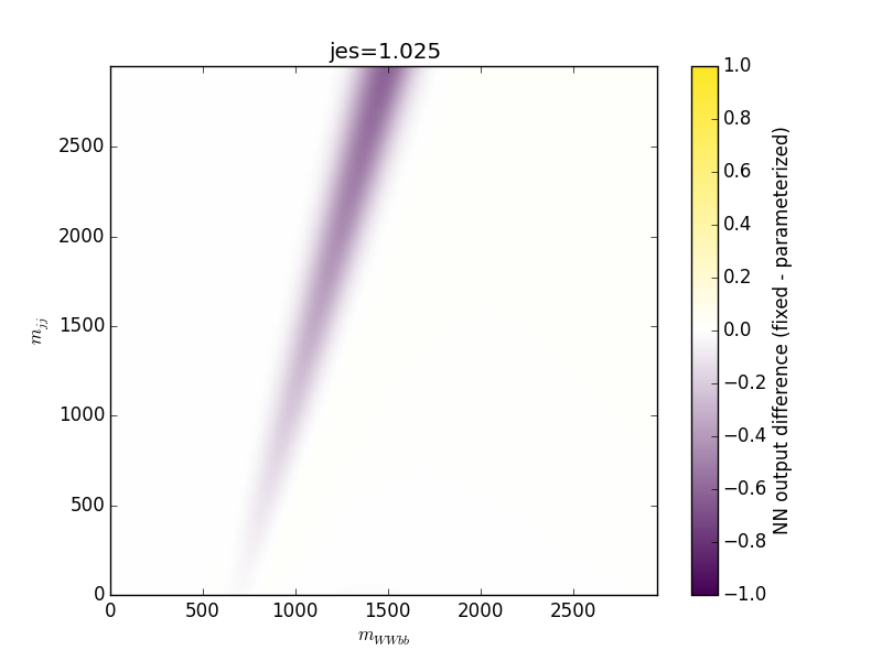
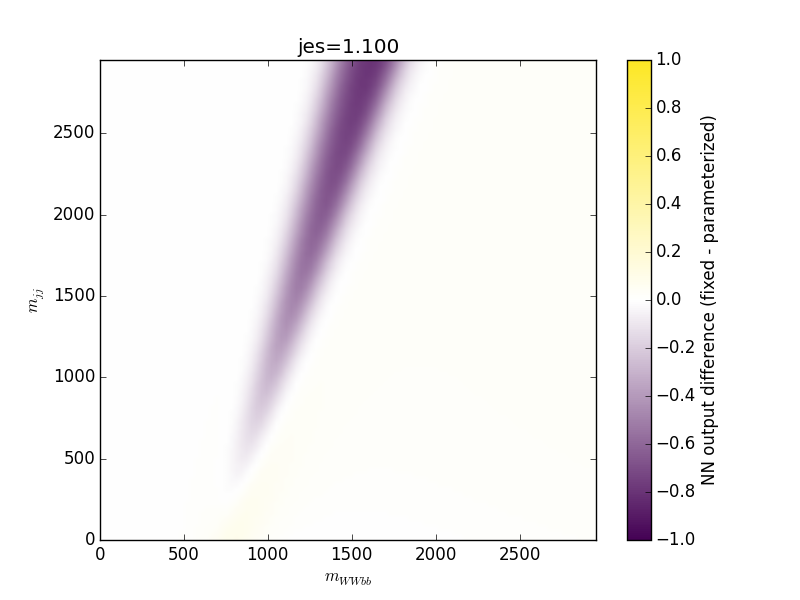
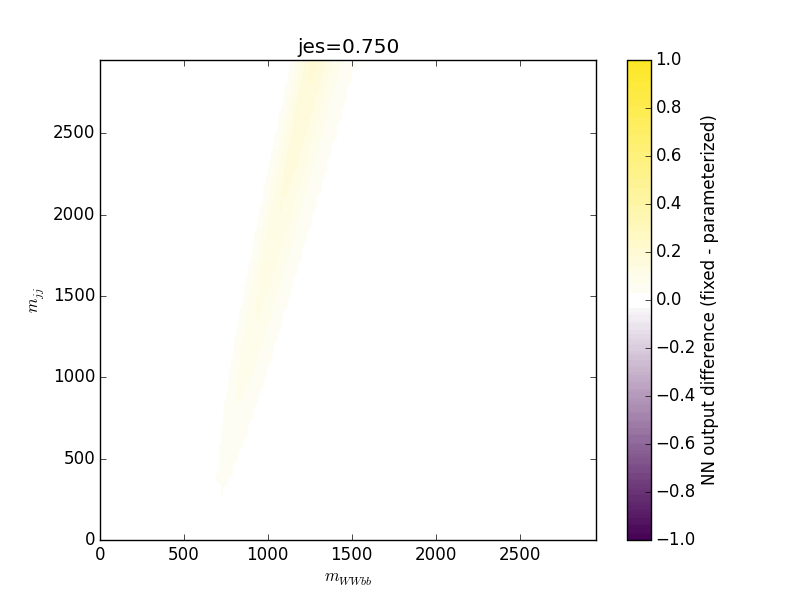
2 mass input values (mWWbb and mjj) are used to train a NN along with jes values of 0.750, 0.900, 0.950, 0.975, 1.000, 1.025, 1.050, 1.100, 1.250.
 |
 |
 |
 |
 |
 |
 |
 |
 |
 |
 |
 |
 |
 |
 |
 |
 |
 |
With 2 input mass values, plotting the NN output requires a 3D plot. This is done using a color-coded heatmap.
 |
 |
 |
 |
 |
 |
 |
 |
 |
Changes in the output as a function of the jet energy scale is subtle but can be easier seen when animated

The same inputs, but interpolated through the parameterized method, yield similar results
 |
 |
 |
 |
 |
 |
 |
 |
 |

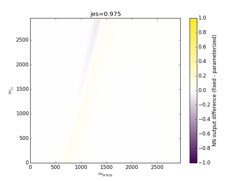
We can track the differences between fixed training and parameterized training method by taking the difference of the two plots.
 |
 |
 |
 |
 |
 |
 |
 |
 |
The Receiver Operating Characteristic can be plotted for both the fixed training and interpolated/parameterized training method