1. Appropriate use of algorithms/models
2. Appropriate explanation for the choice of algorithms/models
3. Appropriate use of evaluation metrics
4. Appropriate explanation for the choice of evaluation metrics
5. Understanding of the different components in the machine learning pipeline

In the src file there will be 2 python scripts namely module1.py and module2.py.

1. module1.py will run and return the results for regression
2. module1.py will run and return the results for classification
3. src file will also include images used for README.MD

Instructions for executing the pipeline and modifying any parameters:

1. Enter into file directory using 'cd (user directory)'
2. Run run.sh by typing 'sh run.sh'
3. run.sh will first install dependent libraries from 'requirements.txt'
4. run.sh will ask for user input to run either module1.py or module2.py

Full insights can be found here. In summary,

1. Dataset is bias to specific State in USA - Washington State
2. Housing prices follows a approximate normal distribution and are skewed to the right
3. Physical features like living_room_size and bathrooms has the biggest corelation to prices
4. Location of house also strongly corelated to prices
5. Date of sale and review has weak corelation

After querying the data from home_sales.db, as null values were only 5-6% of our dataset, we perform simple data cleaning by dropping all null values from our dataset. Afterwards, from the insights we gather from initial data exploration, we feature engineer place_name from zipcode.

We then carry out ordinal encoding by relabel ordinal features - condition and place_name with a numeric value. There might be debate that place_name might be a catagorical feature instead of an ordinal feature. However for this analysis on housing price, solely in Washington State, we discovered a relationship between between place_name and housing prices, hence the decision to use it as an ordinal feature.

After which, I decided to drop date, longitude, id feature as there was no strong correlation to housing price. Due to feature engineering of year and month from date, we had to drop 2923 rows due to misspelling of the months. Doing data exploration, we have came to realized that features sell-year and sell-month does not have a strong enough correalation to justify removing additional 15% of data from out dataset. Hence I will decide to keep it.

Lastly, we perform additional transformation on our dataset to correct skewness by log transforming features that have skewness >0.5 and standardization which make the values of each feature in the data have zero-mean (when subtracting the mean in the numerator) and unit-variance.

credit:Link

We split our data pipeline into train, test and validation splits. Train and test splits will be done using SKlearn library, which split our data into random train and test subsets. Within the train data subset, we will further sample and split our data up to get our validation subset.

credit: Link

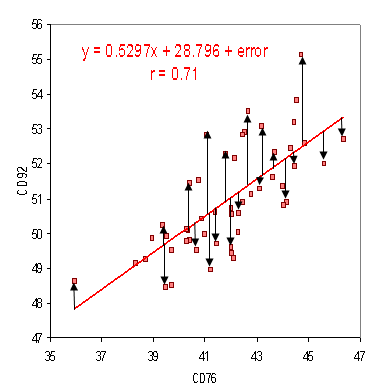
We will be using Root Mean Square Error (RMSE) as the evaluation metrics on the performance of our models. RMSE is the standard deviation of the residuals (prediction errors). Residuals are a measure of how far from the regression line data points are; RMSE measures of how spread out these residuals are. In other words, it tells you how concentrated the data is around the line of best fit.Because we are performing regression, RMSE is a suitable evluation metrics.

credit:Link

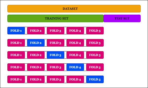
As regression models might be prone to overfitting, we reduce this by performing cross validation using kfold. k-Fold Cross-Validation is a resampling procedure used to evaluate machine learning models on a limited data sample. We will use SKlearn kfold library to perform this procedure.

Taking logs means that errors in predicting expensive houses and cheap houses will affect the result equally. We shall use the log price to train and fit to the regression models. Afterwhich, since the requirements ask that the evaluation metrics be compared with the true house price, we shall convert y_test back to original format before calculating the RSME.

rmse on train 0.2829659844570018 (based on log transformed price) rmse on test 236223.57554988982 (based on true price)

Link here for complete code.

For classification, firstly we have to decide how would we want to bin our house prices. By having fewer bins, we run the risk of can having a misleading histogram. I decided to use a variable bin size according to the 4 quantiles.

1. Bin 0: 0 to 323K
2. Bin 1: 323K to 452K
3. Bin 2: 452K to 650K
4. Bin 3: 650K and above

Normalized Confusion Matrix for GaussianNB
Number of mislabeled points out of a total 9844 points : 4428 accuracy of 0.5501828524989841
Normalized Confusion Matrix for MultinomialNB
Number of mislabeled points out of a total 9844 points : 5343 accuracy of 0.4572328321820398
Normalized Confusion Matrix for SVC
Number of mislabeled points out of a total 9844 points : 4130 accuracy of 0.5804550995530272

Link here for complete code.

1. Standardisation does not have any effect on linear regression models. Standardisation in fact decreased the performance of all 3 classifier models.
2. SVC has the better performance rating