Real estate market is booming, it is particularly true for Budapest, capital city of Hungary, where price of the real estates got multiplied relatively to last years' price. In the current situation individuals are interested in the value of their property, which is pretty difficult to estimate, since it depends on multiple factors.
In this project, I am approaching this problem from supply side by building a machine learning model to estimate fair offer price of the given real estate in Budapest for-sale and for-rent. The output of this project is a supervised offline regression model, which can calculate the offer price of a property based on the given inputs.
- Supervised: desired values are known. e.g. price of the real estates are available
- Offline: the model is not learning real-time, but based on the snapshot of the real estate market
- Regression: predicted value is quasi continuous, in contrast with classification, where the predicted value is category/nominal
At the moment some websites publish average price per square meter of the district and sub-district, where the given property is located.
The machine learning model can be useful for:
- Individuals, who are planning to buy or sell their real estate in Budapest
- Real Estate agencies, for whom knowing the fair offer price is essential
- Detect fradualent activity
I have written a Python script, based on my module real_estate_hungary, which extracts pieces of information from one of the most popular Hungarian real estate website. In short it turns the data on the website into tabular form.
The scraped dataset contains more than 50,000 records of real estate properties in Budapest as of November, 2018.
Locating different attributes of Budapest, such as:
- Boundaries of Budapest and its sub-districts
- Uninhabited areas
- Agglomeration of Budapest
Utilizing overpy a Python wrapper to query geographical data from OpenStreetMap.
GPS coordinates of the properties are available in the scraped data, although elevation of the given coordinate is not published on the real estate website. Luckily some folks put together open-elevation API to make it able to gather elevation data.
Usage is a pretty simple, sending a post request with latitude-longitude pairs and receiving the data in JSON.
For the details and for the code check out the notebook directory in my repository.
After the processing steps:
- Creating a data model by combining the datasets from different sources
- Adding unique composite id
- Extracting numerical values from texts
- Converting features to appropriate data type according to theirs measurement scale
- Splitting the dataset for training and testing set by hash of the id column
Training dataset for respective listing type (for-sale, for-rent):
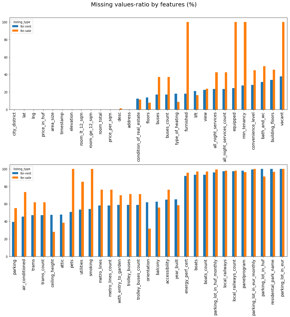
In the scraped dataset, if the user didn't fill in the given attribute of listing property e.g. condition of the real estate, balcony area size etc. then it will appear as missing datapoint. On other hand if a feature is not applicable for the given listing type e.g. in case of properties for sale minimum tenancy, smoking allowed, pets allowed it will appear as missing value as well.
Handling of the missing values:
- No action, using only fully represented variables
- Impute with mean, median, mode
- Model the feature leveraging of other variables
- Using Natural Language Processing on property description and combine with the 3rd option
As a first phase I will use only fully represented features, afterwards I will impute the missing values with predictions of the different models based on NLP, other well-correlated features or the blend of the two.
Fully represented features:
- Price in HUF
- Latitude
- Longitude
- Elevation
- Area size
- Price per square meter
- Total number of rooms, sum of rooms equal or greater than 12 sqm and rooms less than 12 sqm
- District
- Address
The first 7 features measured on ratio scale, others on nominal scale. In machine learning features measured on interval/ratio are preferred.
As a first step, my goal is to create an intuitive machine learning model, from these features. Desirably with only two explanatory variable to be able to visualize in 3D without reducing dimensions.
Building an intuitive Machine Learning model to predict fair offer price of the given property in Budapest
- Dependent variable (predicted): Price per squaremeter
- Explanatory variables (features): GPS coordinates (Latitude, Longitude)
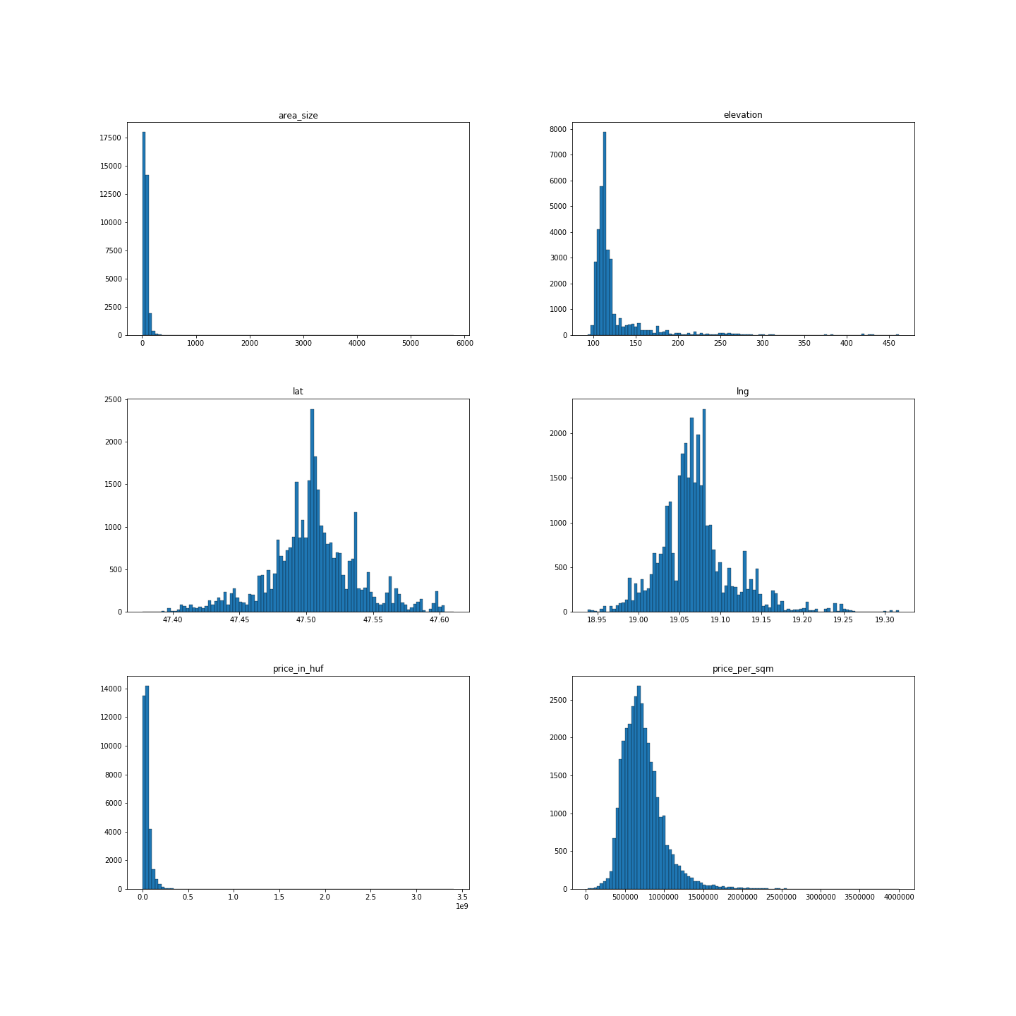
Understand the dynamic of the data, by looking at the distribution of it.
The method I used is z-score or standardization, which is a simple approach to filter out the outliers.
- Standardization:
- Centering the feature by subtracting mean
- Scaling the feature by standard deviation
However this method works well only with quasi normally distributed features, therefore some datatransformation were needed.
Red lines indicates +/- 1 +/- 2 and +/- 3 standard deviation from the mean.

Outliers can be an user input errors or if even they are valid inputs they are not representing well an average real estate in Budapest, therefore the data needs to be normalized by removing outliers.
Based on the five features above, which are greater than 3 SD and less than -3 SD have been removed, therefore 3.34% of the records were removed.

After removing outliers, features have the following estimated distribution. Histogram of Price per square meter, Price and Area size look good, although Latitude and Longitude have some strange spikes, which is worth investigating.

The darker the dot in the map the more properties are listed for sale on the exact spot. It indicates either people want to sell off their apartment under the same address or there are some errors occured during data gathering.
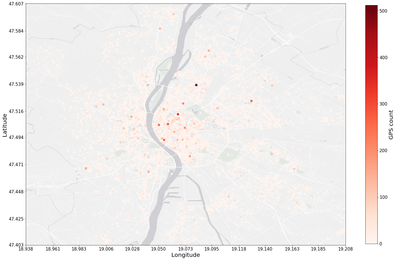
It turned out that these addresses don't contain the street name and the street number, but only the name of the district, sub-district or the residental park name.
The issue with the GPS coordinates is that if the user has not specified the exact address only the district then GPS coordinates point to the center of the district, sub-district. They cover too broad area, consequently longitude and latitude pairs are not accurate enough. These records have been removed with the help of official public domain names such as: street, road, square etc. and defined patterns in regular expression.
After data normalization, I managed to eliminate big spikes in the histogram.

Number of records after data normalization:
- Training set: 23,610, 68.2% of the raw training data
- Testing set: 6,321, 69.1% of the raw testing data
Scatter plots below represent the cross relationship between each feature

Datapoints before fitting the different models, the hotter the point the higher is the Price per square meter in that location. The task is given to fit a surface onto these points, which can predict the price of the real estate most accurately.

For the more details, graphs and code check out the notebook directory in my repository.
- Linear
- Polynomial
- SVM, Gaussian Radial Basis function
- Decision tree
- Random Forest
- Adaptive Boosting
- Gradient Boosting
- K-Neighbours
- Dense Neural Network using Tensorflow, in progress
Building an intuitive Machine Learning model to predict fair offer price of the given property in Budapest
- Dependent variable (predicted): Price per squaremeter
- Explanatory variables (features): GPS coordinates (Latitude, Longitude)
By using only two regressors, it is possible to visualize the decision function in 3 dimensions, without the need of dimension reduction.
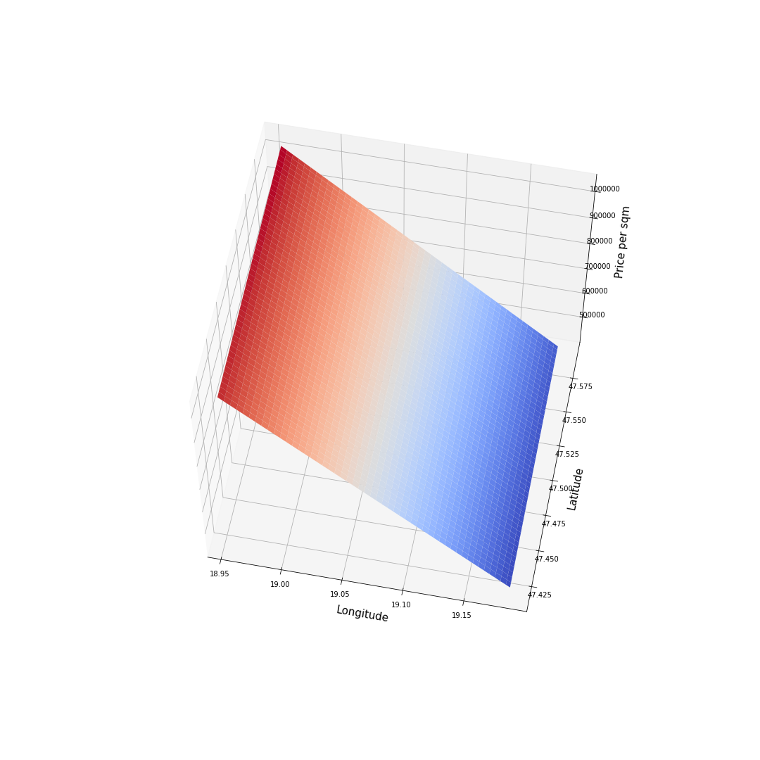
During the Exploratory Data Analysis it was obvious that there is no linear relationship between Price per squaremeter and Latitude, Longitude, but still it is worth checking as the rough estimate. Price per squaremeter is higher on Buda side.
Mean R2 on 10 validation folds: 15.232% with 4.161% standard deviation.
Hyperparameter:
- Degree of polynomial function
After tuning the hyperparameter, the model performs the best with polynomial degree of 9.
Mean R2 on 10 validation folds: 27.295% with 3.640% standard deviation.

Hyperparameters: Kernel: Gaussian Radial Basis function
- C as regularization/smoothing parameter
- Gamma defines kurtosis of the Gaussian curve
Trained two models, difference between them is the level of regularization.
- More regularized, C=10000, Gamma=10: Mean R2 on 10 validation folds: 44.372% with 4.201% standard deviation.

- Less regularized, C=100000, Gamma=100: Mean R2 on 10 validation folds: 49.526% with 4.826% standard deviation. The best estimator after tuning hyperparameters.

Decision Tree Hyperparameters:
- max_depth
- min_samples_split
- min_samples_leaf (leaf_node: pure node, where gini/entrophy = 0)
- min_weight_fraction
- max_features
- max_leaf_nodes
- min_impurity_decrease
- min_impurity_split
After tuning of hyperparameters,
- max_depth=90, max_leaf_nodes=300
Mean R2 on 10 validation folds: 51.125% with 4.843% standard deviation. The CART algorithm is well presented on the surface chart, in which the algorithm keep partitioning dependent variable along the different features. In this case price per square meter has been partitioned by finding the best thresholds in latitude and longitude to generate as homogeneous nodes as it possible.

Ensemble learning method, training 100 decison trees on bootstraped random records of the training data, with the same hyperparamters as decision tree, namely: max_depth=60, max_leaf_nodes=300
Mean R2 on the 'out of bag' validation data: 57.928%.

- Adaptive Boosting
- Gradient Boosting
The idea is the same to train a lot of weak learners to generate ensemble model. Weak learner can be any well regularized model such as SVM, Decision tree. In this case I chose decision tree, since it can be trained pretty fast as opposed to SVM.
Decision tree's hyperparamter: max_depth=10 and number of estimators: 10,000
Mean R2 on 10 validation folds: 47.378% with 4.403% standard deviation.

Decision tree's hyperparamter: max_depth=10 and number of estimators: 100
Mean R2 on 10 validation folds: 55.999% with 4.791% standard deviation.

Hyperparamter:
- k-closest neighbours
After tuning hyperparamter k=92, distance function=euclidean, weights based on the distance i.e. closest datapoint has more effect
Mean R2 on 10 validation folds: 54.805% with 5.249% standard deviation.

For more details and for the code check out the notebook directory in my repository.
All the trained models can be found in model directory of my repository. Calculating the fair offer price of the given real estate in Budapest is pretty easy, all you need:
- Python 3 with installed scikit-learn library
- GPS coordinates of your property, i.e. Latitude and Longitude, you can easily get it from Google Maps
- Area size measured in square meter
import pickleFile path of one of the most accurate model, Random Forest:
filepath_of_the_model = './model/forest_model_57.pkl'Loading the model from disk to python
with open(filepath_of_the_model, 'rb') as f:
    model_obj = pickle.load(f)
Making predictions
- Latitude: 47.498077
- Longitude: 19.0796663
- Area size: 64 square meter
latitude, longitude = 47.498077, 19.0796663
area_size = 64
predicted_price_per_sqm = model_obj.predict([[latitude, longitude]])[0]
print('Based on the location, the fair offer price per square meter: {0:,.0f} Ft.'.format(predicted_price_per_sqm))Based on the location, the fair offer price per square meter: 573,487 Ft.
price = predicted_price_per_sqm * area_size
print('Based on the location and area size, the fair offer price: {0:,.0f} Ft.'.format(price))
Based on the location and area size, the fair offer price: 36,703,153 Ft.
I have listed the best models and run predictions against the unseen testing set.
| Model | R2 on testing set% |
|---|---|
| SVM | 45.63 |
| Decision Tree | 56.58 |
| Random Forest | 58.92 |
| Gradient Boosting | 60.61 |
| K-Neighbours | 60.51 |
The regression model was trained on datapoints listed in Budapest, therefore its predictions are restricted only to the boundaries of the city. Another issue is the uninhabited areas such as the river Danube and the islands along it. At the moment if I feed one of the GPS coordinate of Danube the model will be able to predict price, however it does not make a lot of sense. In order to set the scope of the model a classifier should be trained, which can distinguish among three classes:
- Uninhabited area in Budapest
- Inhabited area in Budapest
- Area outside of Budapest
Scraped dataset and the data queried from OpenStreetMap had sufficient number of distinct GPS coordinates to build a classifier. Training set before model fitting had the following patterns.

Relative occurrences of the classes have been calculated as a benchmark of the classifier, in short the accuracy of the model must be higher than the 83.03% otherwise it underperforms the base estimater based on probalities.
| class | probablity |
|---|---|
| Inhabited area in Budapest | 83.03% |
| Uninhabited area in Budapest | 11.05% |
| Area outside of Budapest | 5.92% |
Selected model is to classify the GPS coordinates into 3 classes is k-neighbours model, with k=1 paramter. By setting the k parameter to 1 the algorithm choses the closest neighbour in the area. Distances calculated by euclidean function. Classifier accuracy is higher that 98% both in the testing set and the validation set, therefore the model outperformed the benchmark.
The classification model is available in the model directory of my repository. The usage is pretty much the same as it was for regression, only the output is the label of the class e.g. 'Uninhabited area in Budapest', 'Inhabited area in Budapest', 'Area outside of Budapest'.
As a demonstration I have looked up two GPS coordinates and feeded it to the model:
- GPS coordinate of the Liberty bridge in Budapest
- Random inhabited area on Buda side
The output can be seen below:
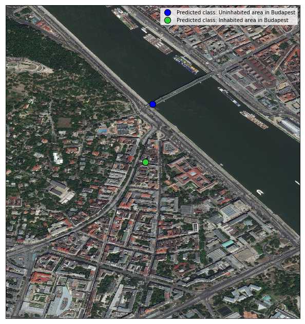
The classification model predicted correct classes. Going forward boundaries of the regression model can be restricted by combining it with the trained classifier.