UCSD Affiliated Research Project Studying Supernova Dust Production in the Small Magellanic Cloud.
This project is written by Bethany A Ludwig and advised by Dr. Karin Sandstrom.

• This is the abridged version. Code has been simplified to save space and to reflect only decisions chosen to remain in the final paper.
• Other methods that were tested but ultimately not used are not contained in this version.
• For a more complete version please email the author.

To run code from scratch, you must install opencv and reproject.

pip install opencv-python reproject

*Assuming python3, may be slightly different for 2.7 ** Note that reproject can be less than predictiable on Windows but appears to run fine on linux.

Contains Infrared images from Spitzer and Herschel which are the primary observations for this project.
Also contains images of E0102 in the Radio and Xray for boundary determination.

The Spitzer 24 micron image has an oversaturated source far away from the remnant that disrupts convolution. This code simply replaces that source with a box of NaNs.

A region in each image at 24 microns (Spitzer) and 70, 100, 160 microns (Herschel) is selected that contains the least (closest to 0) amount of emission in the images while avoiding the edges. The region contains the same RA/DEC coordinates in each image. The median is taken of this region and subtracted from each image. The standard deviation of this region is saved and used later as a source of error during the SED fitting.

Folder contains all Kernels used for convolution. Kernels obtained from Aniano+,2011.
Convolve.py is a convolution module where the master_convolve function can be called in other scripts. The process ensures that the Kernel is equal to one, the max value of the Kernel is in the center, the Kernel array is square. This code isn't built to handle rotation but does flag a warning if rotation needs to be accounted for (i.e. CD1_2 and CD2_1 are nonzero.) This code also doesn't work on rare Kernels that do not contain a single peak intensity in the center.

Mask coordinates are obtained using Chandra Xray data of E0102 at 1100-2000 eV. The data is convolved to the appropriate resolution. The canny edge detection algorithm from opencv2 is used to get the coordinates. The mask is then extended 20 pixels to the left to avoid overcompensating for emission-line nebula N76 during background removal.

E0102 is located within a spatially variable background that must be considered before any measurements can take place.
The four data points we are using to make the measurement include images at 24 microns (Spitzer) and 70, 100, 160 microns (Herschel).

For the 24 and 70 micron images the resolution is good enough that we employ a non linear diffusion based inpainting method to model the background before removing it from the supernova. We apply an iterative solution to Laplace’s equation using backward finite difference in time and second order central difference inspace. I.e.:

To determine when the diffusion process should end, we compare the difference between the sum of the magnitude of the pixel intensities in each time step with the time step that comes immediately after it. When homogenized, there should be no difference between these two time steps so we look for where this subtraction produces 0 within a tolerance of the sky noise error. For 24 microns this is the 1375th step. For 70 microns, this is the 3620th step.

Note that the fits files and movies generated by the code in Background_Removal/Diffusion is not included in this repo to save space. If running from scratch new folders with the correct names will need to be created as they are currently being ignored (folder names can be found in the .gitignore file). Diffusion.py would need to be run before any of the other scripts and does take a while (~30min) to run. This script creates the final modeled background image where the other files are used for visualizing and understanding the results.

Because the 100 and 160 micron images have poorer resolution than 24 and 70, the inpainting method converges too fast and another method should be utilized. To take advantage of all the information in the higher res 70 micron modeled background, we solve for a scale factor between that background and the 100 and 160 images. The scale factor we solve for is based on the median of the ratio of an annulus around the supernova in the background to an annulus around the supernova in the image we are modeling.

We adjust the scale factor to meet the condition that a region, which is generally over subtracted in each image, should ideally be close to zero with any negative intensities the result of noise in the image. We use the median of the ratio as an intial guess and then define a region, centered at RA, DEC = 1h 4m 3.54s -72d 01m 37.55s, with a radius of 3". This is about 4 to 9 pixels depending on the image. This corrects the median by 16% of the initial guess. This adjustment accounts for the fact that there is no constant temperature in the image and that high intensities may be over accounted for in the initial guess.

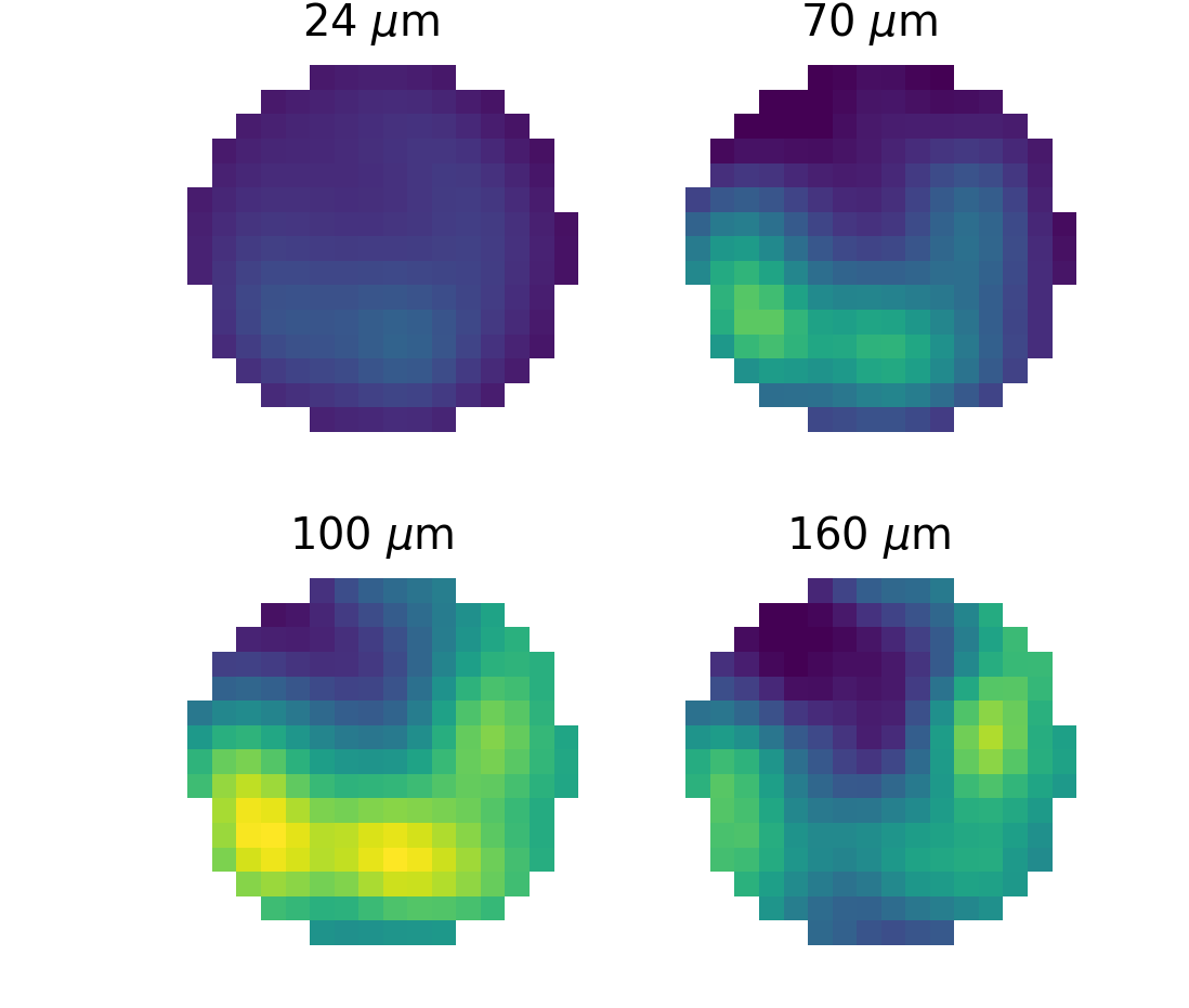
This is the result of all the background removal. The color min and max is the same in all images. This clearly shows why early measurements of E0102 at 24 microns underestimated the amount of dust present in this remnant.

Everything we've done until now has been data reduction, now we take our measurements. We first need to convolve and regrid everything to the lowest resolution, the 160 micron image. We also further reduce the data here by removing everything outside of a 22" radius from the center RA, DEC = 1h 4m 2.1s -72d 01m 52.5s. Files are saved under Final Files and will be used for futher plotting and fitting purposes.

To fit our data to a Spectral Energy Distribution function we need a few equations and modules.
The modified black body equation is given by:

More information about this equation including the derivation and units can be found at Gordon, 2014.

• The kappa variable refers to the emissivity of a dust grain and is dependent on the material and wavelength. For amorphous carbon, our values come from a table by (Rouleau & Martin 1991) and for silicate we use (J ̈ageret al. 2003). Both have a wavelength range up to 104 microns so we extrapolate to 164 microns.
• The Sigma_dust variable is the dust surface mass density given by dust mass * solar mass / physical area. We calculate the physical area of a single pixel in square parsecs to use here. For our integrated solution we will use the area of a single pixel, but for our averaged solution we will use the total area of our supernova remnant.
• The black body equation is given by:

To determine the error we consider during our fit we take a calibration error of 10% across instruments and add it in quadrature to the sky noise that we determined in our sky removal section.

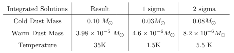
Integrated_SED takes the mean value of the pixel intensities in the subtracted remnant at 24, 70, 100, and 160 microns and fits an SED to those values. The result is a cold dust mass of 0.1 Solar Mass, a warm dust component of 3.98e-05 Solar Mass, and a temperature of 35 K. For convenience, the results and the chi squared confidence intervals of the fit are tabled below.

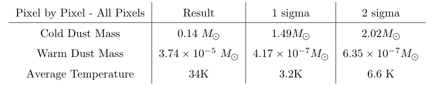
PixByPix_SED fits an SED to each individual pixel in the subtracted remnant at 24, 70, 100, and 160 microns and then totals up the resulting mass estimates. The code is split up into saving the fitted data solutions, including chi squared confidence maps, temperature and mass maps, and then loading those results for evaluation and plotting. The saved solutions take up about 2.4 GiBs and so are not immediately apart of the repo. This code will have to be run before using other code that depends on these solutions.

We consider two solutions here. One with all of the fitted data, the other taking into account that some of the pixel intensities fall below the noise levels, and so may be fit with spurious results.

The error is summed using a frobenius norm, where all the elements in the matrix are squared and summed before the square root is taken. The error in this table is very high because some of the pixels fall below the sky noise level and so are detection limited. They can therefore be fit with spurious errors. In effect, the error of a very small number of pixels dominates the error in all other pixels.

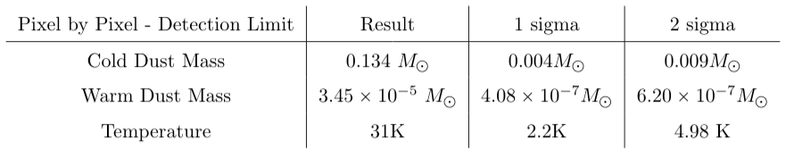
To do this, we create a template where all pixels that are 3 times the noise or higher are set to 1 and all else 0. This template is then multiplied into the solution maps. As a result, the error is reduced significanly as seen in the below table.

During SED Fitting, we are fitting 4 data points with 3 parameters. We save a chi squared map in parameter space and determine the width of the intervals that fall within a confidence level of 1 sigma, or 68.3%. We use the table found in "Numerical Recipes: The Art of Scientific Computing" by William H. Press, 2007.

This is straight forward enough for the integrated SED solution. For the Pixel by Pixel SED solution, all intervals are saved in a map where each pixel in E0102 has an associated chi squared confidence interval for both the cold and warm mass parameters. We then calculate the Frobenius norm of those maps to determine our error. Since we give the temperature solution as an average, and not a sum, we also take the average chi squared confidence interval in points within E0102.

The majority of plots are handled in VisSed.py and require that integrated SED and Pixel by Pixel SED be run prior to its use.

This folder contains the background removed images and those images regridded and convolved to match the resolution of the 160 micron image. It contains the final plots that will be included in the paper.