Dynamic Mode Decomposition

The dynamic mode decomposition (DMD) is an equation-free, data-driven matrix decomposition that is capable of providing accurate reconstructions of spatio-temporal coherent structures arising in nonlinear dynamical systems, or short-time future estimates of such systems. The DMD method provides a regression technique for least-square fitting of video snapshots to a linear dynamical system. The method integrates two of the leading data analysis methods in use today:
Fourier transforms and Principal Components. Originally introduced in the fluid mechanics community, DMD traces its origins to Bernard Koopman in 1931 and can be seen as a special case of Koopman theory. Meanwhile DMD has emerged as a powerful tool for analyzing dynamics of nonlinear systems and in the last few years alone, DMD has seen tremendous development in both theory and application. In theory, DMD has seen innovations around compressive architectures, multi-resolution analysis and de-noising algorithms. In addition to continued progress in fluid dynamics, DMD has been applied to new domains, including neuroscience, epidemiology, robotics, and the current application of video processing and computer vision.

The DMDpack includes the following implementations

• Exact DMD (dmd) facilitating truncated, partial or randomized SVD
• Compressed DMD (cdmd)
• Robust DMD (tdmd) using total least squares

Installation

Get the latest version git clone https://github.com/Benli11/DMDpack

To build and install DMDpack, run from within the main directory in the release: python setup.py install

After successfully installing DMDpack, the unit tests can be run by: python setup.py test

See the documentation for more details.

Example

Get started:

import numpy as np
from dmd import dmd, cdmd
from dmd import tools

First, lets create some (noise-free) toy data:

# Define time and space discretizations
x=np.linspace( -9, 9, 200)
t=np.linspace(0, 3*np.pi , 80) 
dt=t[2]-t[1]
X, T = np.meshgrid(x,t)
# Create two patio-temporal patterns
S1 = 0.9* np.cos(X)*(1.+0.* T)
S2 = ( (1./np.cosh(X)) * np.tanh(X)) *(2.*np.exp(1j*2.8*T))
S= S1+S2

The high-dimensional signal S is superimposed as a time-independent signal S1 and time-dependent signal S2, shown in the following figure:

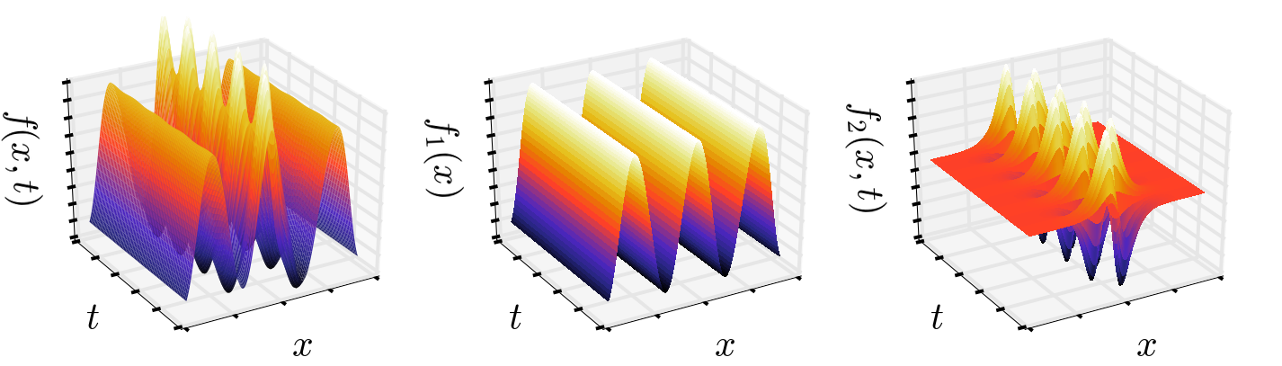
DMD is a data processing algorithm which decomposes a matrix S in space and time. The matrix S is decomposed as S = FBV, where the columns of F contain the dynamic modes. The modes are ordered according to the amplitudes stored in the diagonal matrix B. V is a Vandermonde matrix describing the temporal evolution. Hence, using the dynamic mode decomposition, we aim to separate S into its underlying components, as follows

Fmodes, b, V, omega = dmd(F.T, dt=dt, k=k, return_vandermonde=True, return_amplitudes=True)

Plotting the continuous-time eigenvalues: 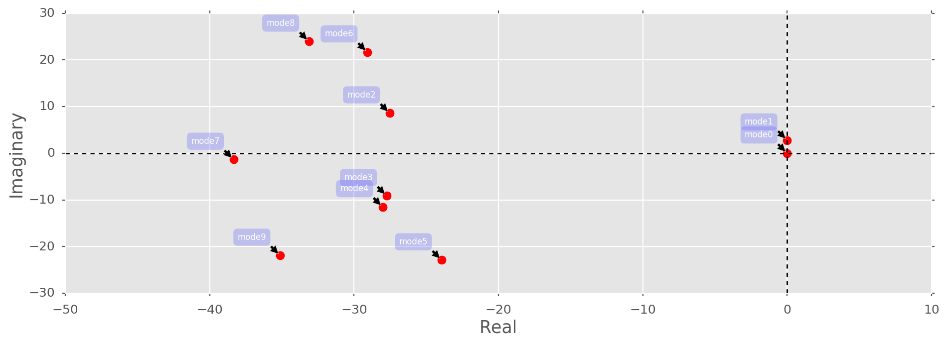we see that S is indeed superimposed from two underlying signals, i.e., mode 1 and 2. All the other modes are bounded far away from the origin and can be considered as unstable, i.e, not relevant for recovering the underlying signals. Hence, we can approximate S, S1 and S2 as follows:

Sre = (Fmodes[:,0:2]*b[0:2]).dot(V[0:2,:]).T
S1re = (Fmodes[:,0:1]*b[0]).dot(V[0:1,:]).T
S2re = (Fmodes[:,1:2]*b[1]).dot(V[1:2,:]).T

Plotting the approximated signals, we indeed capture the underlying signals faithfully

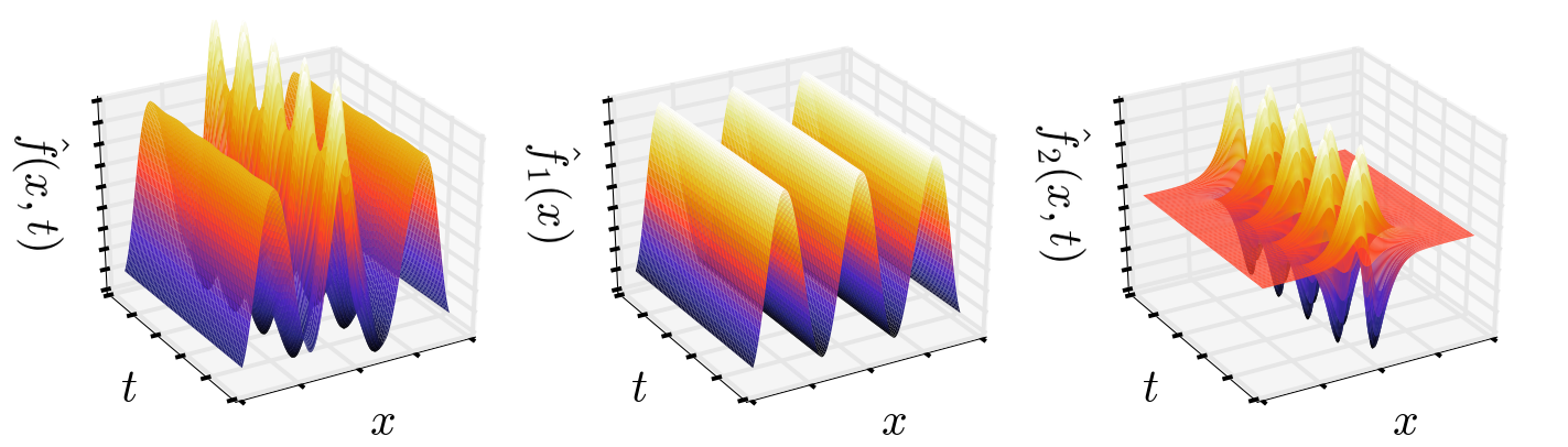
The visual evidence is convincing, let's compute the approximation error in addition:

print(np.linalg.norm(S-Sre, 'fro')/np.linalg.norm(S, 'fro')*100)
print(np.linalg.norm(S1-S1re, 'fro')/np.linalg.norm(S1, 'fro')*100)
print(np.linalg.norm(S2-S2re, 'fro')/np.linalg.norm(S2, 'fro')*100)

which supports the visual evidence

2.82741507892e-12
1.60385599574e-12
4.72877417589e-12