Vehicle detection is an important process in any autonomous driving pipeline. Once the vehicles are identified they can be used to plan how an autonomous vehicle will navigate an enviornment. This will be a tutorial on how to implement a vehicle identifier algorithm using sklearn and OpenCV. The steps of this algortihm are:
- Perform feature extraction on a labeled training set of images and train a classifier.
- Implement a sliding-window technique and use our trained classifier to search for vehicles in images.
- Run our pipeline on a video stream and create a heat map of recurring detections frame by frame to reject outliers and follow detected vehicles.
The first and arguably most important part of a machine learning pipeline is the extraction of good features that provide a rich representation of our objects of interest. We want our classifier to be able to detect cars so we shall use the following features:
- A histogram of oriented gradients (HOG) for each channel.
- A histgram of each color channel.
- A spatial bin of each color channel.
import numpy as np
import cv2
from skimage.feature import hog

def get_hog_features(img, orient, pix_per_cell, cell_per_block,feature_vec=True):

    features = hog(img, orientations=orient,
                   pixels_per_cell=(pix_per_cell, pix_per_cell),
                   cells_per_block=(cell_per_block, cell_per_block),
                   transform_sqrt=True,
                   visualise=False, feature_vector=feature_vec)
    return features

def color_hist(img, nbins=32):
    channel1_hist = np.histogram(img[:,:,0], bins=nbins)
    channel2_hist = np.histogram(img[:,:,1], bins=nbins)
    channel3_hist = np.histogram(img[:,:,2], bins=nbins)
    hist_features = np.concatenate([channel1_hist[0], channel2_hist[0], channel3_hist[1]])
    return hist_features

def bin_spatial(img, size=(32,32)):
    channel1 = cv2.resize(img[:,:,0], size).ravel()
    channel2 = cv2.resize(img[:,:,1], size).ravel()
    channel3 = cv2.resize(img[:,:,2], size).ravel()
    return np.hstack((channel1, channel2, channel3))
For our implemetation we have chosen the following parameters for feature extraction:
- Convert from RGB color space to YCrCb color space
- HOG: 8 oreintation bins, (8,8) pixels pers cell, and 2 cells per block
- Spatial binning dimenstions: (32,32)
- Color Histogram: 32 histogram bins
These parameters were chosen after tuning on multiple test images and seeing which produced the best ratio of true postitives to false positives. Below is an illustration of how HOG differentiates between car and non-car images.

When it comes to choosing a classifier there are a variety of options. Linear Support Vector Machines (SVM) have been shown to work pretty well with HOG features so we'll try that one. As always we split our data into a training and test sets and train on the training set. One feature of SVMs is that they also have a "decision_function" method which can be interpreted as the confidence of our classifier this will be important when we use our classifier to classify new images.
Also before we train our classifier it is important to normalize our features. We do this so that one feature doesnt dominate the others because it just happens to have a broader scale.
from sklearn.svm import LinearSVC
from sklearn.preprocessing import StandardScaler
from sklearn.model_selection import train_test_split

X = np.vstack((car_features, notcar_features)).astype(np.float64)
# Fit a per-column scaler
X_scaler = StandardScaler().fit(X)
# Apply the scaler to X
scaled_X = X_scaler.transform(X)

# Define the labels vector
y = np.hstack((np.ones(len(car_features)), np.zeros(len(notcar_features))))

rand_state = np.random.randint(0, 100)
X_train, X_test, y_train, y_test = train_test_split(
    scaled_X, y, test_size=0.2, random_state=rand_state)

svc = LinearSVC()
svc.fit(X_train, y_train)Now that our classifier is trained we want to classify images in our video stream. To do that we will subsample each image in a region of interest to us into different window sizes and feed them into our classfiier. We'll use 64x64 and 96x96 windows with a bit of overlap as shown below:

What we will find when we test on images is that we get some false positives. We can do a few things to alleviate this problem. One thing is using the "decision_function" from before and thresholding on the returned value. Another thing to notice is that vehicles will be matched in multiple windows in the image. We can define a heat map of these windows and use a threshold to get rid of isolated windows which usually correspond to false positives. Once we have a thresholded heat map we can use a function in scipy called "label" to find the connected regions in our heat map.
from scipy.ndimage.measurements import label

def draw_labeled_bboxes(img, labels):

    for car_number in range(1, labels[1]+1):

        nonzero = (labels[0] == car_number).nonzero()

        nonzeroy = np.array(nonzero[0])
        nonzerox = np.array(nonzero[1])

        bbox = ((np.min(nonzerox), np.min(nonzeroy)), (np.max(nonzerox), np.max(nonzeroy)))

        cv2.rectangle(img, bbox[0], bbox[1], (0,0,255),6)

    return img

def process_image(img_src, vis_heat=False):

    draw_img = np.copy(img_src)
    scales = [1,1.5]
    img_src = img_src.astype(np.float32)/255
    heat_map = np.zeros_like(img_src[:,:,0])

    img_src = cv2.cvtColor(img_src, cv2.COLOR_RGB2YCrCb)
    img_cropped = img_src[y_start_stop[0]:y_start_stop[1],:,:]

    for scale in scales:
        if scale != 1:
            imshape = img_cropped.shape
            img_cropped = cv2.resize(img_cropped, (np.int(imshape[1]/scale), np.int(imshape[0]/scale)))

        ch1 = img_cropped[:,:,0]
        ch2 = img_cropped[:,:,1]
        ch3 = img_cropped[:,:,2]

        nxblocks = (ch1.shape[1]//pix_per_cell) - 1
        nyblocks = (ch1.shape[0]//pix_per_cell) - 1
        window = 64
        nblock_per_window = (window // pix_per_cell) - 1
        cells_per_step = 2
        nxsteps = (nxblocks - nblock_per_window) // cells_per_step
        nysteps = (nyblocks - nblock_per_window) // cells_per_step

        hog1 = get_hog_features(ch1, orient, pix_per_cell, cell_per_block, feature_vec=False)
        hog2 = get_hog_features(ch2, orient, pix_per_cell, cell_per_block, feature_vec=False)
        hog3 = get_hog_features(ch3, orient, pix_per_cell, cell_per_block, feature_vec=False)

        for xb in range(nxsteps):
            for yb in range(nysteps):

                test_features = []
                ypos = yb*cells_per_step
                xpos = xb*cells_per_step
                xleft = xpos*pix_per_cell
                ytop = ypos*pix_per_cell

                subimg = cv2.resize(img_cropped[ytop:ytop+window, xleft:xleft+window], (64,64))
                spatial_features = bin_spatial(subimg, size=spatial_size)
                test_features.append(spatial_features)
                hist_features = color_hist(subimg, nbins=hist_bins)
                test_features.append(hist_features)

                hog_feat1 = hog1[ypos:ypos+nblock_per_window, xpos:xpos+nblock_per_window].ravel()
                hog_feat2 = hog2[ypos:ypos+nblock_per_window, xpos:xpos+nblock_per_window].ravel()
                hog_feat3 = hog3[ypos:ypos+nblock_per_window, xpos:xpos+nblock_per_window].ravel()
                hog_features = np.hstack((hog_feat1, hog_feat2, hog_feat3))
                test_features.append(hog_features)

                test_features = np.concatenate(test_features)
                test_features = X_scaler.transform(test_features)

                test_prediction = svc.decision_function(test_features)

                if test_prediction > 0.75:
                    xbox_left = np.int(xleft*scale)
                    ytop_draw = np.int(ytop*scale)
                    win_draw = np.int(window*scale)
                    heat_map[ytop_draw+y_start_stop[0]:ytop_draw+y_start_stop[0]+win_draw,xbox_left:xbox_left+win_draw] += 1

    heat_map[heat_map <= 1] = 0
    labels = label(heat_map)
    draw_img = draw_labeled_bboxes(draw_img, labels)
Here is a visualization of our heat map and we can clearly see that areas of high intensity correspond to vehicles.

We run this pipeline on each image in our video stream to get this final result. One extra thing I did for our video stream is that I used the heat maps of previous images to get stable boxes around the vehicles. I kept a buffer of 10 heat maps which I summed and thresholded.
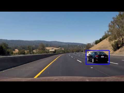
The algortihm is successfully identifying vehicles when they are in range however there is much room for improvement. For future work one could:
- Create a vehicle class and keep track of which pixels are associated with which vehicles.
- A pitfall of the current algortihm is that the classifier was not trained on different weather conditions and that may make it act unpredictably.
- The algorithm can also be further trained to differentiate between vehicle types.