![]()
A graphical application for total X-ray scattering analysis of liquids and amorphous solids.
LiquidDiffract can calculate and refine the normalised structure factor and real-space correlation functions, and extract structural information such as average bond lengths, coordination number, and density.
Benedict J. Heinen (benedict.heinen@gmail.com)
LiquidDiffract is described in an open access paper published in Physics and Chemistry of Minerals:
Please cite this article if you use LiquidDiffract in your work.
- Requirements
- Installation
- Usage
- References
- License
- Python >= 3.5
- SciPy >= 1.2.1
- NumPy >= 1.16.2
- PyQt5 >= 5.12
- pyqtgraph >= 0.10.0
- importlib_resources is required if using Python<3.7
LiquidDiffract should run with earlier versions of these python packages but is untested. LiquidDiffract is system-independent and has been tested on Linux, Mac, and Windows. Dependencies are handled automatically when installing with pip.
The simplest way to install LiquidDiffract is directly from PyPI with pip:
$ python3 -m pip install LiquidDiffract (on Windows use: py -m pip install LiquidDiffract)
The source code is directly available here
We still recommend pip for installing from a local directory. (Invoke setup.py directly at your own risk!)
Development installation
You can make a development (editable) install by using pip's -e flag:
$ pip install -e git+https://github.com/bjheinen/LiquidDiffract#egg=LiquidDiffract
From a local directory:
$ cd /path/to/local/directory/
$ curl -Lo LiquidDiffract.zip https://github.com/bjheinen/LiquidDiffract/archive/master.zip
$ unzip LiquidDiffract.zip
$ mv LiquidDiffract-*/ LiquidDiffract/
$ pip install -e /path/to/local/directory/LiquidDiffract/
This will not actually install anything, but create an .egg-link file in the deployment directory that links to LiquidDiffract's source code.
It is useful if you want to make changes to the source code without having to re-install. Use Python's site-packages directory as the deployment directory if you want your editable install of LiquidDiffract available on your sys.path for other programs using your Python installation. To do this from the github page use the -t flag -t /path/to/directory
To run the software use the command
$ LiquidDiffract
If this fails setuptools may have placed the script in a directory not on your path. The location is usually a user or python specific scripts/bin folder, e.g. /usr/local/bin, ~/anaconda3/bin/, or Python\Python311\Scripts\
Alternatively, run 'ld_launcher.py' from the scripts folder of the installation directory $ python ld_launcher.py
There are four main tabs which provide a selection of toolboxes for data operations at different stages of the workflow.
- Background scaling/subtraction
- Data operations: structure factor calculation, interference function optimisation, and density refinement
- PDF calculation and data output
- Estimation of coordination numbers and bond lengths (integration and curve-fitting)
Data are automatically plotted and tabs updated as operations are made. The graphical plots display coordinates in the upper-right corner. Click and drag or use the scroll-wheel to zoom in on a region. Double right-click to reset the view.

This tab allows data and (optionally) background files to be loaded in. The auto-scale feature speeds up workflow but is not recommended for a close fit.
All data must be in Q-space. A toolbox is provided to convert raw experimental data of 2θ values to Q-space. By default LiquidDiffract expects data in inverse Angstroms, but an option to change this to inverse nano-metres is available in the Additional Preferences dialog, which is accessible from the Tools menu.
This is the tab where most of the data processing takes place.
The sample composition can be set here, along with data processing options. After setting these options the interference function i(Q) is calculated and displayed. i(Q) is related to the total molecular structure factor as:
depending on the formalism used.
This function can then be normalised by minimising errors in the real-space 'differential correlation function', D(r):
In LiquidDiffract the integral in the function D(r) is calculated by taking the imaginary portion of the inverse Fourier transform of Qi(Q) using a standard FFT algorithm.
The sample composition must be set before the structure factor, S(Q), can be calculated. The sample density (in atoms per cubic angstroms) should also be set here. If the density is to be refined, this is used as the initial value passed to the solver.
Spurious peaks or oscillations (e.g. from a slightly mislocated beam stop) in the low-Q region can be removed by setting a Q-min cut-off.
At high Q-values experimental data often becomes increasingly noisy because the relative contribution of coherent scattering to the experimental signal decreases. This increasingly noisy signal can lead to anomalous oscillations near the first peak in D(r). It can therefore be beneficial to truncate the data at high-Q. However truncation can cause spurious peaks in D(r) as a result of the Fourier transform. The positions of these peaks are a function of Q-max, so the use of different values should be investigated. Discussion on the effect of Q-max can be found in ref. [1] and [5].
The option to smooth the data will apply a Savitzky-Golay filter to the data. Options to change the length of the filter window and the order of the polynomial used to fit samples can be found in the Additional Preferences dialog, accessible from the Tools menu.
LiquidDiffract provides the option to use either Ashcroft-Langreth [6] or Faber-Ziman [7] formalisms of the structure factor. See Keen et al., 2001 [8] for discussions of differences in structure factor formalisms, or the LiquidDiffract source code for specific implementations.
In both formalisms the total molecular structure factor, S(Q), is converted to normalised units using the method of Krogh-Moe [9] and Norman [10].
Applying a modification function to S(Q) before FFT can help suppress truncation ripples and can correct a gradient in the high-Q region. Two functions are currently implemented:
Lorch [13]:
Cosine Window (Drewitt et al.) [14]:

where N is width of the window function and x is an integer with values from 0 : (N-1) across the window
After calculating the structure factor the final tab can be used to output S(Q), the pair distribution function, g(r), and the radial distribution function, RDF(r), as is.
The numerical iterative procedure used by LiquidDiffract to minimize the error in the determination of g(r) follows the one proposed by Eggert et al., 2002 [1-4]. This procedure is based on the assumption that a minimum distance, r-min, can be defined, which represents the largest distance (0 -- r-min) where no atom can be found. In a liquid, this should be the region within the 1st coordination shell. Because no atom can be present in this region, no oscillations should be observed in the g(r) function. As a result, the function D(r < r-min) = -4πrρ However oscillations are commonly observed in this region, due to the effect of an experimentally limited Q-range (Q-max < &inf;), and systematic errors in the scattering factors and normalisation factor, α. The iterative procedure calculates the difference between real and model data in the low-r region and scales S(Q) accordingly to reduce this.
To refine S(Q) the value of r-min should be set carefully, as it has a strong influence. The position of r-min should correspond to the base of the first coordinence sphere in the g(r).
The number of iterations in the procedure can also be set; a minimum of 3 is normally required for convergence.
A Χ2 figure of merit, defined as the area under the curve ΔD(r) for r<r-min, is used to rate the refinement.
Where,
The sample density and/or background scaling factor can be determined by finding the values of ρ and or b that provides the best convergence of the iterative procedure described above. This is done by minimising the resultant value of Χ2. LiquidDiffract supports several different solvers to do this. The solver in use, along with specific options like convergence criteria and number of iterations, can be selected from the Additional Preferences dialog. The solvers currently supported are:
-
L-BFGS-B [16-17]
-
SLSQP [18]
-
COBYLA [19-21]
All solvers require upper and lower bounds on the density and or background scaling factor to be set.
The density and background scaling factor can be refined independently or simultaneously.
For more information on these optimisation algorithms please see the SciPy documentation, or consult the references listed.
The optimisation algorithms used to estimate density work best when the initial guess, ρ0 is close to the true value. If the density of the material is very poorly known it is recommended to use the global optimisation option provided. It is not recommended if a good initial guess can be made, due to slower, and sometimes poor, convergence.
The global optimisation procedure used is the basin-hopping algorithm provided by the SciPy library [22-23]. Basin-hopping is a stochastic algorithm which attempts to find the global minimum of a function by applying an iterative process with each cycle composed of the following features:
- random perturbation of the coordinates
- local minimization
- accept or reject the new coordinates based on the minimized function value
The acceptance test used here is the Metropolis criterion of standard Monte Carlo algorithms [23].
For more information see the SciPy documentation, or consult the references listed.
It is important to note that a well defined minimum in Χ2n only exists for n <~ 10. This is a result of how the iterative procedure works, and the definition of Χ2.
More info...
The Eggert method works by forcing the region below rmin to fit a line defined as -4πρr. Χ2n is the square of the area between this modelled line and D(r) (r < rmin) after n iterations. Χ2(ρ) should display a minimum when the slope (controlled by density) best fits the data. However, after a large number of iterations the data can always be forced to fit the model slope through unreasonable manipulation (e.g. by massively inflating low-Q values), and so Χ2n will be drastically reduced at large values of n. Furthermore, at large values of n, Χ2n will decrease as ρ --> 0, because the absolute values used to calculate Χ2 are smaller as the magnitude of the slope decreases.
We can investigate this by computing the function Χ2n(ρ, n) - in this case for an example composition with a density ~0.048 atoms per cubic Angstrom. Plotting Χ2n(ρ) for n = 4 and n = 25 shows that with only 25 iterations there is no longer a well defined minimum.

As n increases, the density region in which the eggert algorithm can fit the data to the model is rapidly increasing too:

The range of value of n that result in a well defined minimum will depend on the data (or more properly on the rmin value used). This change in the behaviour of Χ2n(ρ, n) can best be illustrated by plotting the double natural logarithm of normalised Χ2 values, because the magnitude of Χ2n(ρ, n) is so much lower at large n, and the minima in the function much shallower. For this data it takes 3 iterations for the procedure to converge properly, after which there is a clear stable minimum which allows an accurate density estimate to be retrieved. Above 10 iterations the method no longer works, because of a sharp shelf in the function.
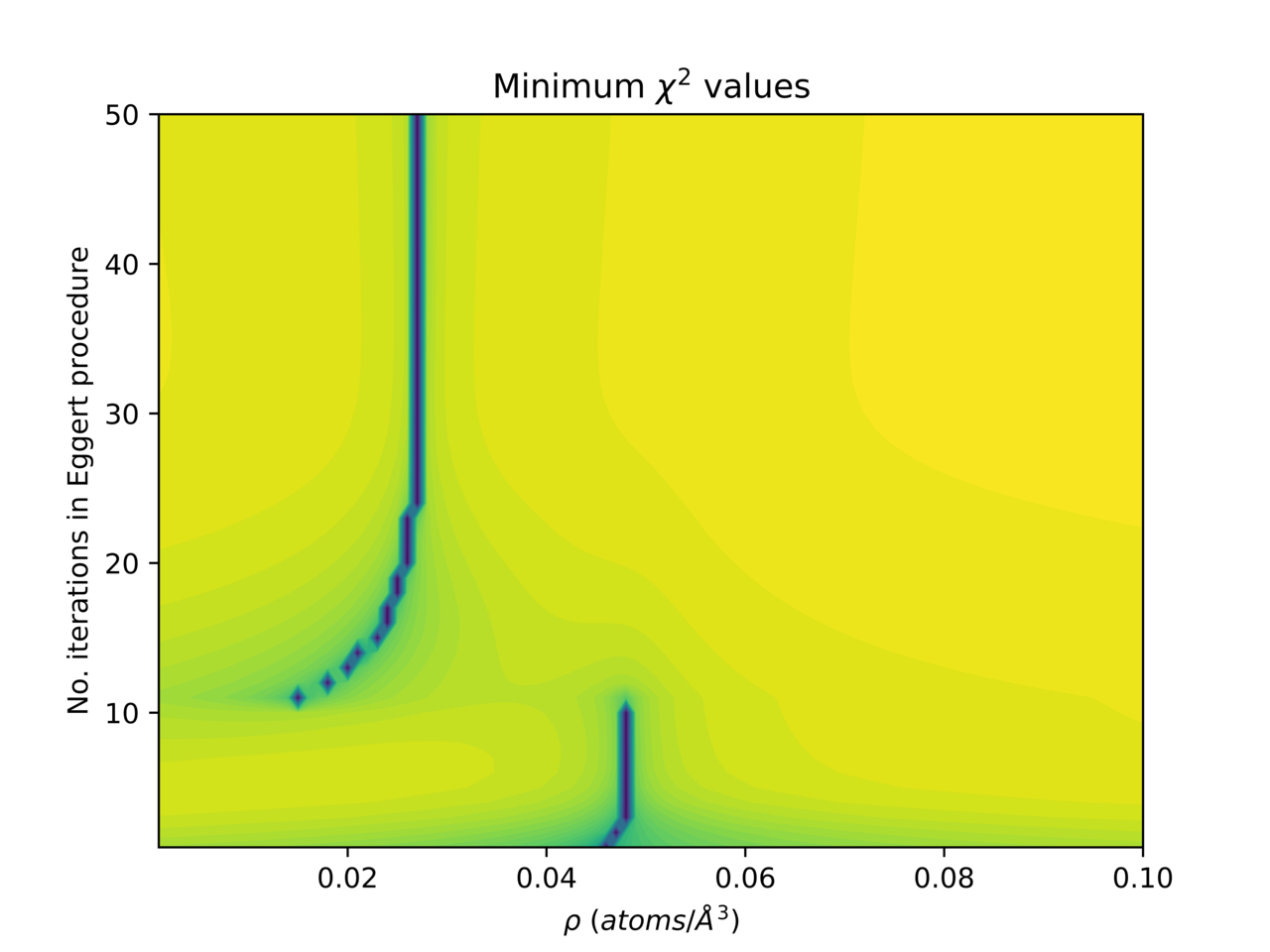
At high enough resolution the number of iterations can be optimised. For this particular data it is 7.

A log is automatically generated for any refinement made. This log includes information on the data file, sample composition, data and refinement options used, solver output/convergence info (if refining density), and the final Χ2 and ρ.
The log for each refinement is automatically written to file. The default behaviour is to store each log in a file named 'refinement.log' within the current data directory. Each log is preceded by a time-stamp. The log-mode can be changed to Overwrite in the Additional Preferences dialog. This creates a new log file for each data file loaded, which will be overwritten if already present. The file-names generated are of the form 'DATAFILENAME_refinement.log' and are similarly created in the source directory of the loaded data file.
LiquidDiffract outputs some density refinement information to the terminal. There is an option provided to print convergence progress messages to the terminal also. This can be useful for real-time monitoring (e.g. when using the slow global optimisation with a known number of iterations).
The third tab displays the optimised S(Q), g(r), and RDF(r). The buttons at the bottom of the window allow each one to be saved to a text file. If a modification function has been used in the data treatment then information on this will also be saved, along with the raw S(Q).
g(r) is the pair-distribution function. It is defined as:
Where the interference function, i(Q) is:
RDF(r) is the radial distribution function:
its integration across peaks yields atomic coordination numbers.
D(r)
The density function, D(r), that is used in the data analysis and defined above, should not be confused with g(r) or RDF(r). In the literature it is sometimes referred to by other names, including F(r), G(r), and PDF(r). It is defined as:
This tab provides tools to extract coordination numbers and average bond lengths from the RDF(r). Two toolboxes are provided, an integration toolbox which does simple integration across peaks in the RDF(r) for monatomic samples, and a curve-fitting toolbox which allows the user to fit the RDF(r) with an arbitrary number of weighted gaussian-type peaks.
Integrating across the peaks in RDF(r) gives the average coordination number. Three methods for doing this are provided based on those commonly used in the literature [24]. The first method is based on the assumption that the quantity rg(r) is symmetrical for a coordination shell about its average position. The second method is based on the assumption that the coordination shell is instead symmetrical about a radius which defines the maximum in the r2g(r) curve. Since the first peak is not truly symmetrical NA and NB can be considered estimates of the lower bound on the coordination number. Typically it also the case that NA < NB. This consideration of asymmetry leads to the third method, which involves integrating RDF(r) from the leading edge of the first peak r0 to first minimum following it, rmin.
An auto-refine button is provided to quickly find the positions of r0, r'max, rmax and rmin using a root-finding and minimisation procedure. The user can also set the limits manually via a spinbox or by dragging the limits on the data plot. In particular, careful setting of rmin may be required as its apparent value can fluctuate due to errors in RDF(r) [25].
For polyatomic samples it is more useful to fit the RDF(r) with a number of peaks so that the individual contribution from different α-β pairs can be investigated [26-27]. LiquidDiffract provides a curve fitting toolbox to do this. Either the RDF(r) or the T(r) can be fitted, with T(r) defined as:
LiquidDiffract fits the data with an arbitrary number of gaussian type peaks (with an optional skewness parameter) based on the function:
The x-ray weighting factors are computed automatically and the fitting parameters are the coordination number, Nαβ, the bond length, rαβ, and a measure of the bond length distribution, σαβ. The skewness parameter, ξ, is optional in the fit. All of the parameters can be set manually and individually toggled between remaining fixed or allowed to vary in the fit.
The module LiquidDiffract.core.core is the core library which provides all the specific functions for processing (liquid) diffraction data. This can be imported and used in your own Python code. There are also some data helper functions (e.g. to rebin data) found in LiquidDiffract.core.data_utils
A brief example of using LiquidDiffract in a custom data processing script is given below:
Example usage
#!/usr/bin/env python3
# -*- coding: utf-8 -*-

# Import required python modules
import numpy as np
# Import optional python modules used in this example
import matplotlib.pyplot as plt

from scipy.optimize import minimize
# import the LiquidDiffract core module
import LiquidDiffract.core.core as liquid
import LiquidDiffract.core.data_utils as data_utils

# First set composition
# The composition should be a dictionary dictionary with short element names as keys,
# and values as tuples of the form (Z, charge, number_of_atoms)
# The file 'example_data.dat' contains background corrected total scattering data of Gallium at high pressure
composition = {'Ga': (31,0,1)}
# Set initial density - in atoms per cubic Angstrom
rho = 0.055

# Load data
# LiquidDiffract expects x data to be Q values in Angstroms (not nm!)
# The file 'example_data.dat' has already been background corrected
q_raw, I_raw = np.loadtxt('example_data.dat', unpack=True, skiprows=0)

# Next rebin data and trim if necessary
# Re-bin via interpolation so dq (steps of q) is consistent to allow FT
# This can be done using the rebin_data function from core.data_utils
dq=0.02
q_data, I_data = data_utils.rebin_data(q_raw, I_raw, dx=dq, x_lim=[q_raw[0], 11.8])

# Apply any other data treatment
# e.g. a savitsky-golay filter to smooth the data
I_data = data_utils.smooth_data(I_data, method='savitzky-golay',
                                window_length=31, poly_order=3)

# First calculate the interference function i(Q)
# i(Q) = S(Q) - S_inf (S_inf = 1 for monatomic samples, or in the Faber-Ziman formalism)
structure_factor = liquid.calc_structure_factor(q_data, I_data, composition, rho, method='faber-ziman')
interference_func = structure_factor - liquid.calc_S_inf(composition, q_data, method='faber-ziman')

# store original interference function
interference_func_0 = interference_func

# A low r region cutoff must be chosen for the refinement method of Eggert et al. (2002)
# A density value in atoms(or molecules) / A^3 must also be set. This will be
# used as the starting estimate if the density is refined.
r_min = 2.3
rho_0 = rho

# The function 'calc_impr_interference_func' calculates an improved estimate of
# the interference function via the iterative procedure described in Eggert et al., 2002.
#
# calc_impr_interference_func requires the following arguments:
# q_data - q values
# I_data / i(Q) - the treated intensity data or interference function (depends on opt_flag used)
# composition - composition dictionary
# r_min - low r cut-off
# iter_limit - iteration limit for Eggert procedure
# method - method of calculating S(Q) ('ashcroft-langreth' and 'faber-ziman' are currently supported)
# mod_func - modification function to use ('None', 'Cosine-window' or 'Lorch')
# window_start - window_start of cosine function (if in use)
# fft_N sets the size of the array during the fourier transform to 2**N
# opt_flag - set to 0 if not running from solver
#
# The last positional argument (opt_flag) signals that you only want the chi_squared value to be returned.
# This is useful if using a solver to refine the density by minimising the chi_squared value

# e.g.
# Return the improved i(Q) & chi^2 at density = rho_0
iter_limit = 25
method = 'faber-ziman'
mod_func = 'Cosine-window'
window_start = 7
fft_N = 12
args = (q_data, interference_func_0, composition, rho_0,
        r_min, iter_limit, method, mod_func, window_start, fft_N)
# Store the refined interference function at rho_0
interference_func_1, chi_sq_1 = liquid.calc_impr_interference_func(*args)

# Next we pass the function calc_impr_interference_func to
# a solver to estimate the density. We use a separate objective function
# core.redinement_objfun to make this simpler.
# The argument opt_rho is set to 1 to indicate we are refining the density
opt_rho = 1
# The argument opt_bkg is set to 0 to indicate we are not refining
# the background sclaing factor.
opt_bkg = 0
# When refinind the density an iter_limit <= 10 is recommended
iter_limit_refine = 7
args = (q_data, I_data, composition, r_min,
        iter_limit_refine, method,
        mod_func, window_start, fft_N,
        opt_rho, opt_bkg)
# Set-up bounds and other options according to the documentation of solver/minimisation routine
bounds = ((0.045, 0.065),)
op_method = 'L-BFGS-B'
optimisation_options = {'disp': 0,
                        'maxiter': 15000,
                        'maxfun': 15000,
                        'ftol': 2.22e-12,
                        'gtol': 1e-12
                        }
opt_result = minimize(liquid.refinement_objfun, rho_0,
                      bounds=bounds, args=args,
                      options=optimisation_options,
                      method=op_method)
# The solver finds the value of rho that gives the smallest chi^2
rho_refined = opt_result.x[0]

# The interference function can then be re-calculated using the new value for rho,
# and the F(r) refined as above.
interference_func = (liquid.calc_structure_factor(q_data,I_data, composition, rho_refined) -
                     liquid.calc_S_inf(composition, q_data))

args = (q_data, interference_func, composition, rho_refined,
        r_min, iter_limit, method, mod_func, window_start, fft_N)
interference_func_2, chi_sq_2 = liquid.calc_impr_interference_func(*args)

# Calculate the corresponding pair distribution functions g(r)
r, g_r_0 = liquid.calc_correlation_func(q_data, interference_func_0, rho_0, dx=dq,
                                        mod_func=mod_func, window_start=window_start,
                                        function='pair_dist_func')
# r values will be the same
_, g_r_1 = liquid.calc_correlation_func(q_data, interference_func_1, rho_0, dx=dq,
                                        mod_func=mod_func, window_start=window_start,
                                        function='pair_dist_func')
_, g_r_2 = liquid.calc_correlation_func(q_data, interference_func_2, rho_refined, dx=dq,
                                        mod_func=mod_func, window_start=window_start,
                                        function='pair_dist_func')

# Plot the data
fig1 = plt.figure()
plt.xlabel(r'Q ($\AA^{-1}$)')
plt.ylabel(r'i(Q)')
# Initial interference function calculation
plt.plot(q_data, interference_func_0, color='g', label=r'Initial i(Q) | $ρ = {rho:.2f}$'.format(rho=rho_0))
# Optimised at rho_0
plt.plot(q_data, interference_func_1, color='r', label=r'Optimised i(Q) | $ρ = {rho:.2f}$ & $χ^{{2}} = {chisq:.2f}$'.format(rho=rho_0, chisq=chi_sq_1))
# Optimised, using refined density estimate
plt.plot(q_data, interference_func_2, color='b', label=r'Optimised i(Q) | $ρ = {rho:.3f}$ & $χ^{{2}} = {chisq:.2f}$'.format(rho=rho_refined, chisq=chi_sq_2))
# Add a legend
plt.legend(loc='best')
# Show the plots
plt.show()

fig2 = plt.figure()
plt.xlabel(r'r ($\AA$)')
plt.ylabel(r'g(r)')
plt.ylim((np.nanmin(g_r_2), np.nanmax(g_r_2)))
window = len(q_data)
# Initial g(r)
plt.plot(r[:window], g_r_0[:window], color='g', label=r'Initial g(r) | $ρ = {rho:.2f}$'.format(rho=rho_0))
# Optimised g(r) at rho_0
plt.plot(r[:window], g_r_1[:window], color='r', label=r'Optimised g(r) | $ρ = {rho:.2f}$ & $χ^{{2}} = {chisq:.2f}$'.format(rho=rho_0, chisq=chi_sq_1))
# Optimised g(r), using refined density estimate
plt.plot(r[:window], g_r_2[:window], color='b', label=r'Optimised g(r) | $ρ = {rho:.3f}$ & $χ^{{2}} = {chisq:.2f}$'.format(rho=rho_refined, chisq=chi_sq_2))
# Add a legend
plt.legend(loc='best')
# Show the plots
plt.show()[1] Eggert, J. H., Weck, G., Loubeyre, P., & Mezouar, M. (2002). Quantitative structure factor and density measurements of high-pressure fluids in diamond anvil cells by x-ray diffraction: Argon and water. Physical Review B, 65(17), 174105.
[2] Morard, G., Siebert, J., Andrault, D., Guignot, N., Garbarino, G., Guyot, F., & Antonangeli, D. (2013). The Earth's core composition from high pressure density measurements of liquid iron alloys. Earth and Planetary Science Letters, 373, 169-178.
[3] Decremps, F., Morard, G., Garbarino, G., & Casula, M. (2016). Polyamorphism of a Ce-based bulk metallic glass by high-pressure and high-temperature density measurements. Physical Review B, 93(5), 054209.
[4] Kaplow, R., Strong, S. L., & Averbach, B. L. (1965). Radial density functions for liquid mercury and lead. Physical Review, 138(5A), A1336.
[5] Shen, G., Rivers, M. L., Sutton, S. R., Sata, N., Prakapenka, V. B., Oxley, J., & Suslick, K. S. (2004). The structure of amorphous iron at high pressures to 67 GPa measured in a diamond anvil cell. Physics of the Earth and Planetary Interiors, 143, 481-495.
[6] Ashcroft, N. W., & Langreth, D. C. (1967). Structure of binary liquid mixtures. I. Physical Review, 156(3), 685.
[7] Faber, T. E., & Ziman, J. M. (1965). A theory of the electrical properties of liquid metals: III. The resistivity of binary alloys. Philosophical Magazine, 11(109), 153-173.
[8] Keen, D. A. (2001). A comparison of various commonly used correlation functions for describing total scattering. Journal of Applied Crystallography, 34(2), 172-177.
[9] Krogh-Moe, J. (1956). A method for converting experimental X-ray intensities to an absolute scale. Acta Crystallographica, 9(11), 951-953.
[10] Norman, N. (1957). The Fourier transform method for normalizing intensities. Acta Crystallographica, 10(5), 370-373.
[11] Hubbell, J. H., Veigele, W. J., Briggs, E. A., Brown, R. T., Cromer, D. T., & Howerton, D. R. (1975). Atomic form factors, incoherent scattering functions, and photon scattering cross sections. Journal of physical and chemical reference data, 4(3), 471-538.
[12a] Brown, P. J., Fox, A. G., Maslen, E. N., O'Keefe, M. A., & Willis, B. T. M. (2006). 'Intensity of diffracted intensities' in International Tables for Crystallography, Vol. C., ch. 6.1, pp. 554-595
[12b] This form factor data is also available freely at: http://lampx.tugraz.at/~hadley/ss1/crystaldiffraction/atomicformfactors/formfactors.php
[13] Lorch, E. (1969). Neutron diffraction by germania, silica and radiation-damaged silica glasses. Journal of Physics C: Solid State Physics, 2(2), 229.
[14] Drewitt, J. W., Sanloup, C., Bytchkov, A., Brassamin, S., & Hennet, L. (2013). Structure of (FexCa1−xO)y(SiO 2)1−y liquids and glasses from high-energy x-ray diffraction: Implications for the structure of natural basaltic magmas. Physical Review B, 87(22), 224201.
[15] Morard, G., Garbarino, G., Antonangeli, D., Andrault, D., Guignot, N., Siebert, J., Roberge, M., Boulard, E., Lincot, A., Denoeud, A. & Petitgirard, S. (2014). Density measurements and structural properties of liquid and amorphous metals under high pressure. High Pressure Research, 34(1), 9-21.
[16] Byrd, R H and P Lu and J. Nocedal. 1995. A Limited Memory Algorithm for Bound Constrained Optimization. SIAM Journal on Scientific and Statistical Computing 16 (5): 1190-1208.
[17] Zhu, C and R H Byrd and J Nocedal. 1997. L-BFGS-B: Algorithm 778: L-BFGS-B, FORTRAN routines for large scale bound constrained optimization. ACM Transactions on Mathematical Software 23 (4): 550-560.
[18] Kraft, D. A software package for sequential quadratic programming. 1988. Tech. Rep. DFVLR-FB 88-28, DLR German Aerospace Center – Institute for Flight Mechanics, Koln, Germany.
[19] Powell, M J D. A direct search optimization method that models the objective and constraint functions by linear interpolation. 1994. Advances in Optimization and Numerical Analysis, eds. S. Gomez and J-P Hennart, Kluwer Academic (Dordrecht), 51-67.
[20] Powell M J D. Direct search algorithms for optimization calculations. 1998. Acta Numerica 7: 287-336.
[21] Powell M J D. A view of algorithms for optimization without derivatives. 2007.Cambridge University Technical Report DAMTP 2007/NA03
[22] Wales, D J, and Doye J P K, Global Optimization by Basin-Hopping and the Lowest Energy Structures of Lennard-Jones Clusters Containing up to 110 Atoms. Journal of Physical Chemistry A, 1997, 101, 5111.
[23] Li, Z. and Scheraga, H. A., Monte Carlo-minimization approach to the multiple-minima problem in protein folding, Proc. Natl. Acad. Sci. USA, 1987, 84, 6611.
[24] Waseda, Y. The Structure of Non Crystalline Materials: Liquids and Amorphous Solids. 1980. McGraw-Hill, New York
[25] Yagafarov O F, Katayama Y, Brazhkin V V, Lyapin A G, and Saitoh H. Energy dispersive x-ray diffraction and reverse monte carlo structural study of liquid gallium under pressure. 2012. Physical Review B, 40286(17):174103
[26] Petkov, V. Pair Distribution Functions Analysis. 2012. American Cancer Society, doi.org/10.3861002/0471266965.com159
[27] Sukhomlinov S V, and Muser, M H. Determination of accurate, mean bond lengths from radial distribution functions. 2017. The Journal of chemical physics, 146(2):024506
Licensed under the GNU General Public License (GPL), version 3 or later.
See the license file for more information.
This program comes with absolutely no warranty or guarantee.
Copyright © 2018-2022 – Benedict J Heinen