Clone the repository from pycloak. Then in the pycloak top-level directory,

python setup.py install

• numpy
• matplotlib

This package is designed to solve the a particular active control problem in two dimensions for the homogeneous Helmholtz equation. Mathematical details are presented in the included pdf file, readme-overview.pdf. This software was written initially in order to yield numerical results for a recent research paper. As such, it includes a variety of modules and routines designed to set up the general framework of the problem, allowing for manipulation of many different domain parameters and coefficients. Once the problem is set up properly using the ControlProblem class, one can use tikhonov_solve from regsolve.py in order to find a given solution.

1. antenna.py

• Antenna - Generic class for an antenna object
• Rectangle - Rectangular shaped antenna object
• PolarArray - Multiple antenna array object, where each antenna has the same parametrization in polar coordinates with a different center.
• Polar - A single antenna defined in polar coordinates and with center at the origin

2. controlregion.py

• ControlRegion
• AnnularSector
• Rectangle

3. dlpotential.py

• ControlProblem - General framework for setting up the control problem with an Antenna object, two ControlRegion objects, boundaryfunction.Source or boundaryfunction.PointSource object, and other relevant parameters for discretization
• helmholtz_fs - Computes the fundamental solution for the Helmholtz equation at given points
• ddn_helmholtz_fs - Computes the normal derivative to the fundamental solution on boundary of Antenna object
• ddn_helmholtz_fs_j - Computes the normal derivative on the j^th connected component of a antenna.PolarArray object

4. boundaryfunction.py

• Source - Generic class for a source function
• PointSource - A source function which is described as a point source
• PlaneWave - A source function that is represented as a plane wave
• trace - evaluates the boundary function on the boundary of a given ControlRegion object

5. regsolve.py

• tikhonov_solve - Solves for the regularized boundary solution phi at discrete points on the Antenna object which yields the desired control within the specified tolerance parameters.

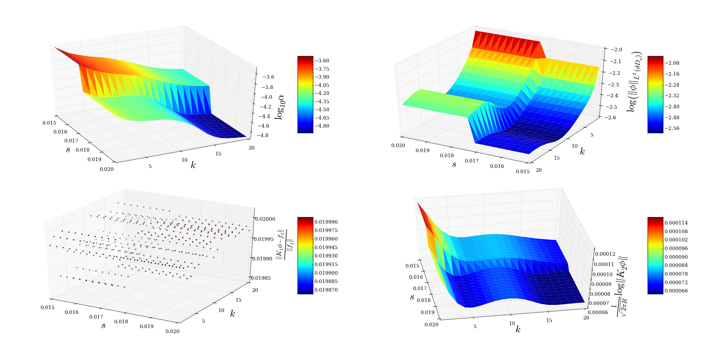
1. plot_s_k - Provides template to plot data from array_linear_vary_s_k.py experiment routine
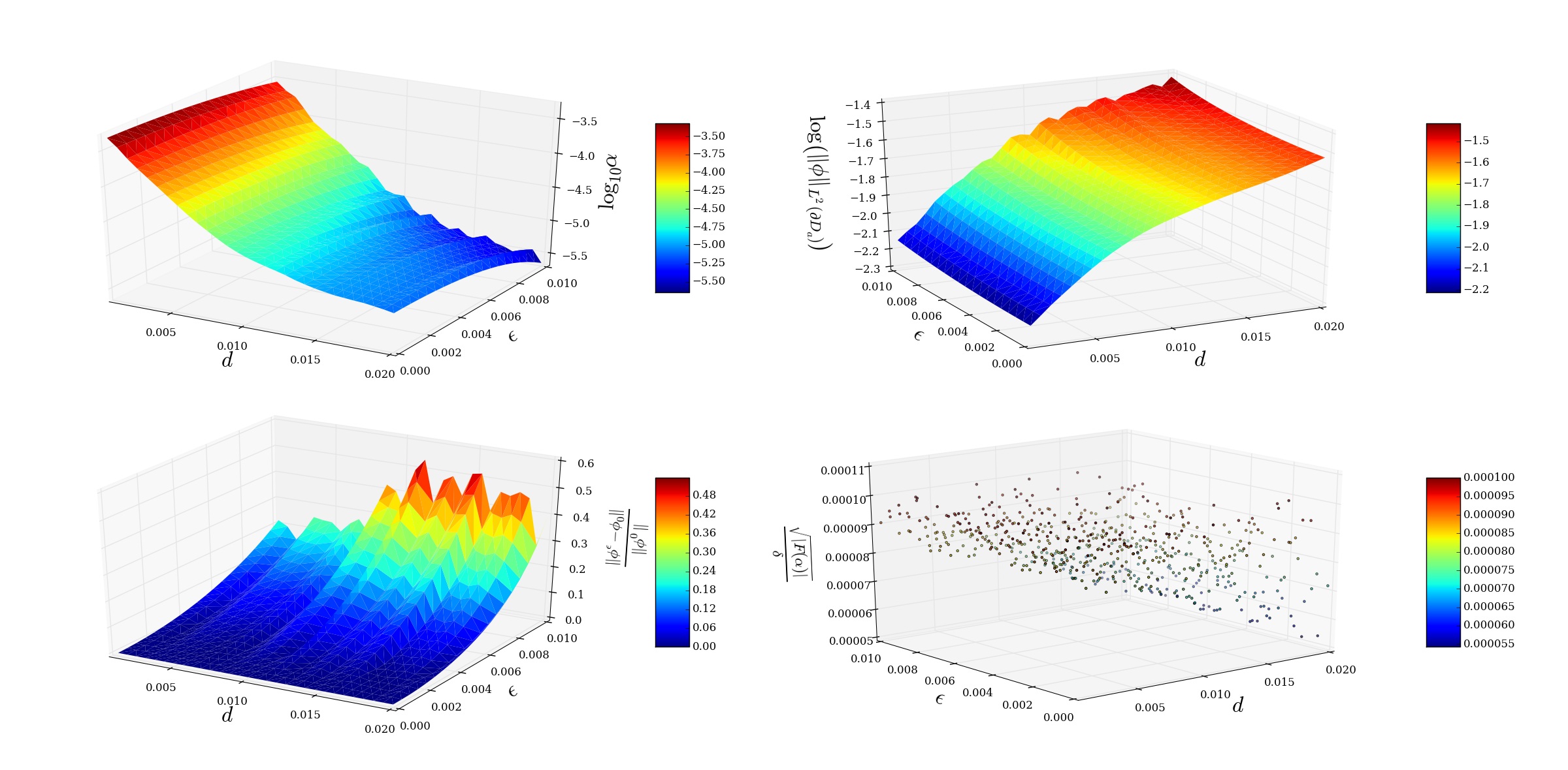
2. plot_d_epsilon - Provides template to plot data from polar_vary_d_epsilon.py experiment routine

1. guicloaker.py
2. visuals.py

1. Here the control region is an annular sector defined by 0.011 <= r <= 0.015 and a = 0.01 is the radius of a circular antenna centered at the origin. The aperture of the control region is spanned from 3pi/4 <= theta <= 5pi/4. We take the incident field to be cancelled out to be a point source originating from x0 = (10000, 0). Then we vary the distance d = r1 - a from 0.001 to 0.02 while keeping r2 - r1 = 0.004 a constant. We add noise to the incident field with a noise level varying in the range 0 <= epsilon <= 0.01. The specified tolerance for cancellation of the incident field for each case is set to be delta = 0.02.
   One can generate the data for this experiment by inputting the following from within the pycloak/experiments directory:
   $ python polar_vary_d_epsilon.py
   Once this completes input
   $ python plot_polar_vary_d_epsilon.py polar_vary_d_epsilon_data.npz
   
2. Similarly, we can conduct an experiment where the control region is a rectangle with lower left corner at (-0.021, -0.1), width 0.01, and height 0.2. This time the antenna is an array of circular antennas arranged vertically, each with radius a = 0.01. The spacing between antenna is given by s > 0 and one antenna is centered at the origin. We then vary the spacing between the antenna elements while adjusting how many there are in order to ensure that the array spans the entire width of the control rectangle. We also vary the wave number k over the interval [1, 20].
   One can generate the data for this experiment by the following:
   $ python linear_array_vary_s_k.py
   Once this is complete, input
   $ python plot_linear_array_vary_s_k.py linear_array_vary_s_k_data.npz