NOTES:

1. The script for running the code as done by me in preparing this assignment, is written to be used in IPython ¹. A detailed session (with outputs as well, is given in session.ipy)
2. This document has some equations that require javascript to run, and an internet connection (to http://orgmode.org/ for the functions).

I used this code: #+INCLUDE “code/hw2.py” src python :lines “1-17”

#+INCLUDE “code/session.ipy” src python :lines “5-14”

And got this scatter plot (Figure 1):

I used #+INCLUDE “code/hw2.py” src python :lines “19-30”

and ran #+INCLUDE “code/session.ipy” src python :lines “16-38”

to get Figure 2

but this seemed a bit to small of an error, so I also ran: #+INCLUDE “code/session.ipy” src python :lines “39-56”

to get Figure 3:

Which I feel makes the point of over-fitting more obvious.

Using the standard penalty function:

\begin{equation} E_W(w) = \frac{1}{2} W^T⋅ W = \frac{1}{2} ∑_m=1^MW_m² \end{equation}

and the given solution to the penalized least-squares problem: \begin{equation} W_PLS = (Φ^TΦ + λ \mathrm{I})^-1Φ^Tt \end{equation}

I wrote: #+INCLUDE “code/hw2.py” src python :lines “31-46”

To generate the 3 slices of the data set: #+INCLUDE “code/hw2.py” src python :lines “47-59”

To get the error term for given $x_i$, $t_i$ $M$ and the normalized error function, for the training and other sets:

#+INCLUDE “code/session.ipy” src python :lines “57-82” Producing:

#+INCLUDE “code/session.ipy” src python :lines “84-116”

My conclusion is that (as pointed out in class) choosing the $λ$ value that minimizes the error on the validation set, is a good heuristic to the value that will minimize the test set. Therefore, I wrote LoptimizePLS(xt, tt, xv, tv, M) such that it will choose the $λ$ that has the minimal error on the validate set. It’s also worth mentioning that a $λ$ value greater than 1 is not very helpful.

#+INCLUDE “code/hw2.py” src python :lines “87-104”

To return the following equations:

\begin{equation} m(x) = \frac{1}{σ²} Φ(x)^T S ∑_n=1^NΦ(x_n) t_n \end{equation}

\begin{equation} var(x) = S²(x) = σ² + Φ(x)^T S Φ(x) \end{equation}

\begin{equation} S^-1 = α I + \frac{1}{σ²} ∑_n=1^NΦ(x_n)Φ(x_n)^T \end{equation}

The implementation is: #+INCLUDE “code/hw2.py” src python :lines “106-128”

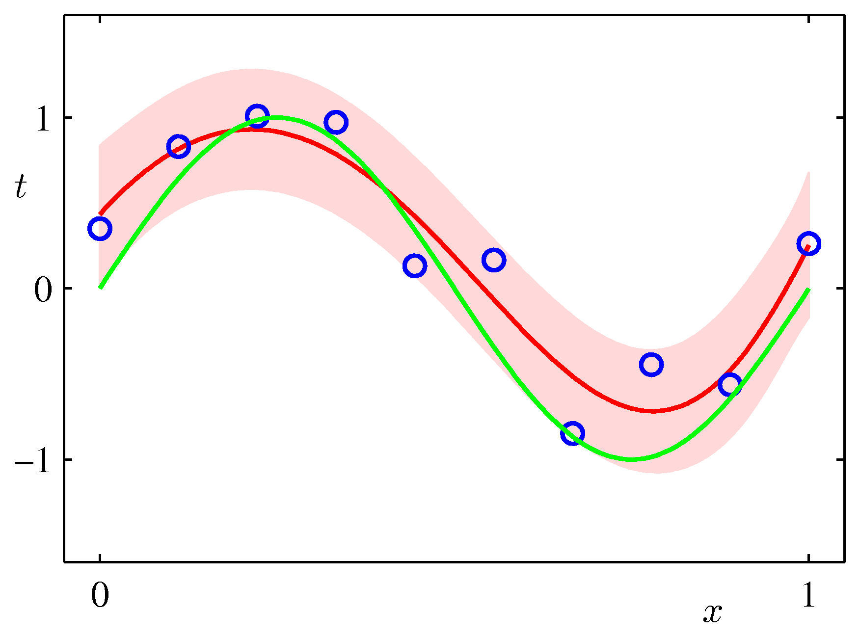
running: #+INCLUDE “code/session.ipy” src python :lines “112-127” resulted in Figure 4:

and for $N=100$: #+INCLUDE “code/session.ipy” src python :lines “112-127” resulted in Figure 5:

BUT Bishop used $sin(2 π x)$ which looks nicer, so I tried that too: #+INCLUDE “code/session.ipy” src python :lines “147-183”

We should notice that in contrast to bishop (see below), in our graph, the $σ²$ values visibly decrease on ‘linear’ parts of the sinusoidal, and increase on ‘curved’ ones.

¹ Fernando Pérez, Brian E. Granger, IPython: A System for Interactive Scientific Computing, Computing in Science and Engineering, vol. 9, no. 3, pp. 21-29, May/June 2007, doi:10.1109/MCSE.2007.53. URL: http://ipython.org