QUICKFIT is an interactive tool for fitting kinetics profiles from profile diagnostics on tokamaks. It presents several advantages compared to conventional tools. Profiles are fitted by 2D Gaussian processes, which allows for better utilize experimental data even for non-stationary or fast-evolving profiles. Further, data fetching, mapping, and fitting sequences usually take just several seconds for the whole discharge. Therefore, the tool is suitable for the fast preview of radial profiles in the control room as well as for the careful and detailed preparation of inputs to other codes.

DIII-D, NSTX, Alcator C-mod, ASDEX Upgrade

The QUICKFIT module is available in the OMFIT framework. It allows the preparation of experimental input profiles for other modules like kineticEFITtime, TRANSP, IMPRAD, KN1D, NEO, and FIDASIM. Support for other modules can be included if requested.

1. Start the python GUI by module load quickfitand quickfit or from as a QUICKFIT module in OMFIT.
2. Select a shot number and kinetic profile to be loaded.
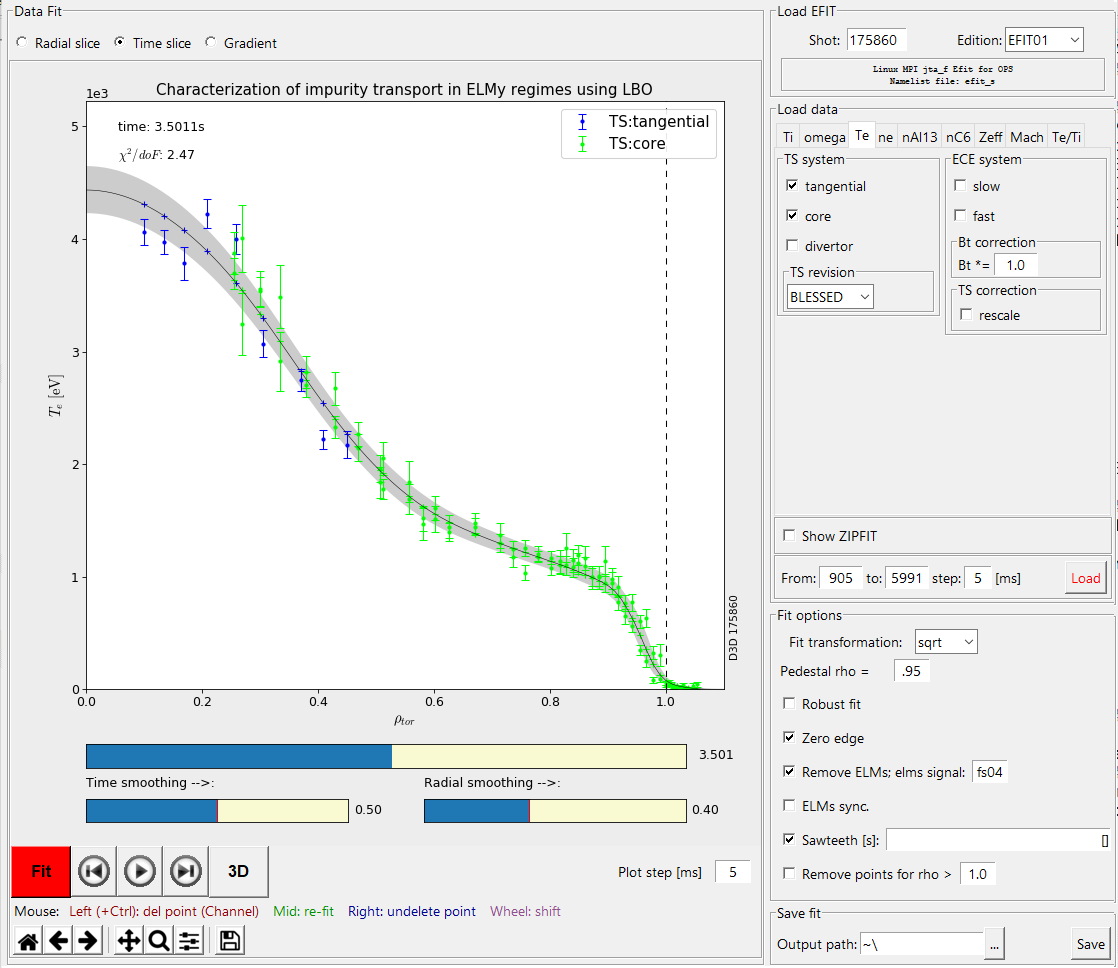
3. If you are satisfied with the default fit options, press the red button FIT in lower-left corner of the GUI or use the middle mouse button to click on the plot. Data can be saved by Save button.
4. More detailed option selection can be done in the right panel. EFIT is specified in frame Load EFIT. Then in frame Load data select a panel with the desired quantity for a fitting and specify which diagnostics systems should be loaded. Further, specify the time range for the loading and the timestep (if empty, it will determine the optimal time step based on the diagnostic timebase).
5. The Fit options can specify a fitting method's configuration. Fit transformation maps data before fitting to improve the fit of peak profiles or force positivity (sqrt, log). Help can be found by placing a mouse above the option in GUI. The time and radial smoothing can be modified by sliders on the bottom left of the window.

• The left part of the window is dedicated to visualizing the experimental data and profile fits. It is controlled via buttons on the bottom of the GUI, a left/right arrow keyboard button, or a mouse. The mouse wheel shifts the profile fit in time, and the middle mouse button recalculates the fit. Double+click or dragging by a left/right mouse button remove/recover data points. When Ctrl is pressed, all data from the selected channel will be removed/recovered. The entire diagnostic can be removed/recovered by mouse click on the legend.

• On the top left of the window can be specified the view type - time slice, radial slice, or normalized gradient. The width of the time window used for plotting is specified by Plot time [ms]. This option is not changing the temporal resolution of the fit.

• When the fit is done, check all time frames carefully, remove all corrupted measurements and try to optimize radial and temporal smoothing. And check all three views (radial, temporal, gradient) to avoid unpleasant surprises later.

Output can be saved as Numpy .npz file, which can be later loaded in OMFIT or used directly. If the QUICKFIT is loaded as the OMFIT module, the data are saved directly to OMFITtree root['OUTPUTS'].