Vol Surface Parametrisation

Ngrok link to the dashboard: https://vol.ngrok.io/

About

My initial goal was to find a robust way of generating arbitrage-free volatility surface on single stock options quotes so that I would be able to determine the change in portfolio liquidation value for change in moments of volatility, spreads, cost of carry, price of underlying, and time. I have decided to use Gatheral's Surface Stochastic Volatility Inspired (SSVI) method for this but had few issues with poor fit. This was expected as I was using volatility derived from american option quotes which volatility explode in wings due to early exercise premium inflating relative value. So instead of direct minimisation on raw volatilities, I had to first de-americanise them by deducting the premium they command with respect to european quotes.

For this, I went along with Kim integral approximation method instead of trees, as it has a very useful feature of decomposition of american options value into european base and early exercise values. However, as this method involves a numerical solution of quadrature formulas on each step exercise boundary, even with Numpy vectorisation and broadcasting it was still quite slow. So I wrote the quadrature pricer class in C++ and used Ctypes library to call its functions from Python. Having derived de-americanised volatilities, I was able to minimise on quotes directly, which has significantly reduced errors in fit.

Calibration to the market is done using SLSQP algorithm with constraints and bounds to prevent arbitrage on the surface. Risk neutral density is derived using fitted SSVI parameters with explicit differentiation of BSM formula and primes of surface function. I have changed Jump-wing parameters from 5 to 3 where we now have ATMF volatility, skew, and kurtosis which we can shock and invert back to raw parameters to get the new volatility surface.

All the above is packed into Numpy structs to allow for better handling of multi-dimensionality and memory optimisation, for example in the case of plotting payoffs and liquidation values with respect to change in underlying and time. I have used Plotly and Ipwidgets packages for the interface, and have deployed a notebook using Voila that I have tunneled to public access using Ngrok.

Features

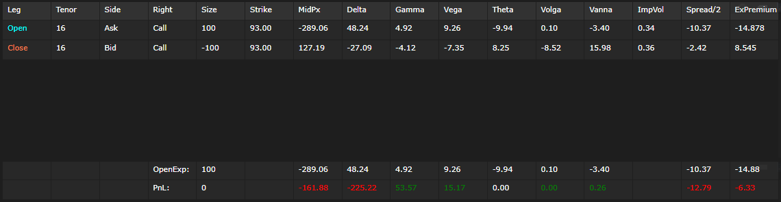
Breakdown of positions liquidation value by Greeks, Spread, and EEP for given changes in 11 factors by expiry group.
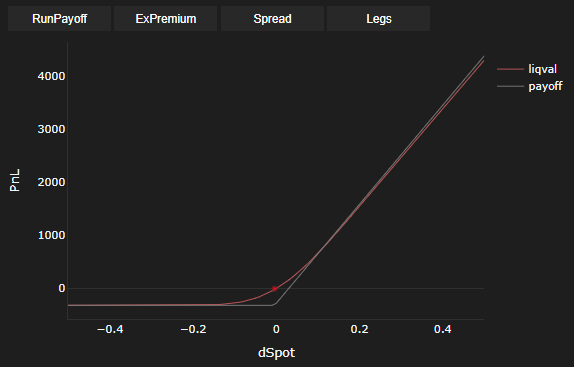
Plotting of payoffs and values for dS and dT ranges that use the factor changes as specified by the user and consider Spread and EEP.
Density and total variance plots for referring to the absence of arbitrage within the newly generated surface specified by the user.
Daily data with the 10-minute interval for 40 listed US single stock option names, with 3 front-month expiries per each where available.
Ability to specify weights for the SSVI fit residual based on gaussian density location and scale parameters.

Guide

Select ticker, trade date, time and click Load.

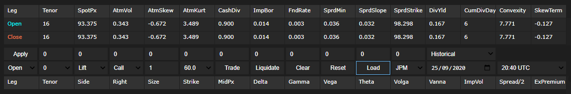
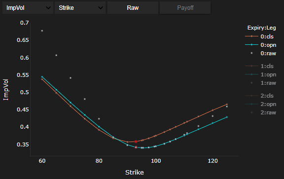
Graphs will show up as the one below, where cyan is yaxis corresponding to open leg and orange for close leg - which we will adjust via changes to params in 3.

We can go ahead and adjust params. In this case we decrease SpotPx by 5% and increase AtmVol by 5% for expiry group 0. Click Apply to make changes.

Select compare data on hover on the vol graph (two bars on upper rhs). Once satisfied with selected strike, right, expiry and side; lift Call 93 expiry group 0 in this case - click.

Red dots will appear corresponding to selected strike for open and close leg in this case.

This will also populate table as below, showing breakdown for the selected strike.

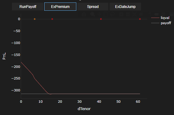
To get pnl range for change in SpotPx click RunPayoff on the buttom lhs graph.

To get pnl range for change in Tenor click RunPayoff on the buttom rhs graph.

Changes in factors will reflect on all graphs, below one is risk neutral density for example. As you can see increasing atm vol flattens the distribution. Use this as guide to adjust surface so long as density is non negative at any point (or else this is butterfly arbitrage) and total variance never intersects (or else this is calendar arbitrage).

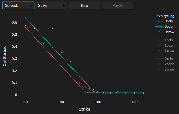
We can select different measure for yaxis and xaxis for upper graphs, in the below example we switch to Spreads, and see that we paid less for on liquidation vs initiation. This is because we have simulated a 5% decrease in SpotPx and spreads widen the deeper ITM option is: so here we Kh has adjusted as per the spot move 1.05 * Kh. This behaviour can be overriden in by changing corresponding parameters, SprdStrike for Kh in this case.

Formulas

Vol Calibration

SSVI fits on total ATMF variance (θ) and logstrike (k) space, where we can specify a type of convexity function (φ) and spot-vol correlation function (ρ):

$w(k) = \frac{\theta_{t}}{2}(1 + k\rho(\theta_{t})\phi(\theta_{t}) + \sqrt{(k\phi(\theta_{t}) + \rho(\theta_{t}))^2 + (1-\rho(\theta_{t})^2)})$

$k = K/F_{T}$

$\rho(\theta_{t}) = ae^{-b\theta_{t}} + c$

$\phi(\theta_{t}) = \eta\theta_{t}^{-\lambda}$

Then we need to minimise the below residual:

$\sigma_{ssvi} = \sqrt{w(k,\theta_{t},\phi,\rho)/t}$

$\epsilon = arg min(\sigma_{ssvi} - \sigma_{quotes})^2$

Risk Neutral Density

Explicit differentiation of BSM formula leads to:

$g(k) = (1-\frac{kw'(k)}{2w(k)})^2-\frac{w'(k)^2}{4}(\frac{1}{w(k)} + \frac{1}{4}) + \frac{w''(k)}{2}$

Where we need to find 1st and 2nd derivatives of total variance wrt logstrike, so we just take these from the surface function w(k):

$w(k) = \frac{\theta}{2}[1 + k\rho\phi + \sqrt{(k\phi + \rho)^{2} (1 - \rho^{2})}]$

$w(k){}' = \frac{\theta}{2}[\frac{k\phi^2 + \rho\phi}{\sqrt{(k\phi + \rho)^2 - \rho^2 + 1} + \rho\phi}]$

$w(k){}'' = -[ \frac{\theta\phi^2(\rho^2-1)}{2((k\phi + \rho)^2-\rho^2 + 1)^\frac{3}{2}} ]$

And to get probability density:

$d_{-}(k) = -\frac{k}{\sqrt{w}}\frac{\sqrt{w}}{2}$

$p(k) = \frac{g(k)}{\sqrt{2\pi w(k)}}e^{-\frac{d_{-}(k)}{2}^2}$

Jump-wings

Jump-wings I have used are a bit different from the ones proposed by Gatheral, but the principle and the goal are the same. We want to know how will vol surface behave if we change 3 vol factors: level (σ), skew (ψ) and kurtosis (κ).

Converting from raw to jw:

$\sigma_{t} = \sqrt{\theta/t}$

$\psi_{t} = [ \frac{1}{2}\rho\phi\sqrt{\theta}]/t$

$\kappa_{t} = [ \frac{1}{2}\phi^2\theta(1 - \rho^2))]/t$

Converting from jw to raw:

$\theta_{t} = \sigma^2t$

$\rho = \frac{\psi t}{\sqrt{\frac{\kappa t}{2} (\psi t)^2}}$

$\phi= \frac{2\psi t}{\rho\sqrt{\theta}}$

Spread function

We fit the the below functions on the raw spreads to get the three parameters:

$H_{Call}(S) = H_{0} + H_{1}max(S-K_{h},0)$

$H_{Put}(S) = H_{0} + H_{1}max(K_{h}-S,0)$

Spread widens for deeper ITM options, we make no assumption here as to where it starts to widen, but Kh should be around ATM/F.

H0: minimum spread H1: slope the spread climb Kh: strike of spread climb

American options value

Is composed of european base value and early exercise premium (EEP):

$C(S,T) = c(S,T) + EEP_{Call}(S,T)$

$P(S,T) = p(S,T) + EEP_{Put}(S,T)$

European options value:

$c(S,T) = Se^{-qT}N(d1(S,K,T))-Ke^{-rT}N(d2(S,K,T))$

$p(S,T) = Ke^{-rT}N(-d2(S,K,T))-Se^{-qT}N(-d1(S,K,T))$

Where EEP is the integral of the boundary price (B) from present till the expiry (T):

$EEP_{Call}(S,T) = \int_{0}^{T} [qB_{t}e^{-q(T-t)}N(d1(S,B_{t},T-t))-rKe^{-r(T-t)}N(d2(S,B_{t},T-t))] dt$

$EEP_{Put}(S,T) = \int_{0}^{T} [rKe^{-r(T-t)}N(-d2(S,B_{t},T-t))-qB_{t}e^{-q(T-t)}N(-d1(S,B_{t},T-t))] dt$

Boundary conditions

Boundary price is the price at which returns from selling options and execising it are the same, and is subject to below conditions.

Terminal condition:

$B_{T,Call} = Kmax(1,\frac{r}{q})$

$B_{T,Put} = Kmin(1,\frac{r}{q})$

High-contact condition:

$\lim_{S\rightarrow B_{t}} \frac{\partial P(S,K,t)}{\partial S} = -1$

$\lim_{S\rightarrow B_{t}} \frac{\partial C(S,K,t)}{\partial S} = 1$

Value-matching condition:

$\lim_{S\rightarrow B_{t}} P(S,K,t) = K - B_{t}$

$\lim_{S\rightarrow B_{t}} C(S,K,t) = B_{t} - K$

Boundary solution

We derive boundary via backward induction where we start at expiry and move through backwards in time. As per Terminal condition we can already find out what is the boundary on the expiry date.

$B_{t} - K = c(B_{t},T-t) + EEP_{Call}(B_{t},T-t) - H(B_{t})$

$K - B_{t} = p(B_{t},T-t) + EEP_{Put}(B_{t},T-t) - H(B_{t})$

Note that we deduct half-spread from the above to adjust the difference in liquidity between the spot and option, in addition to the fact that spread widens as options gets deeper ITM which is exactly where the boundary is located.

We use Trapezoid rule to find the quadrature for the EEP component and final value as we integrate all the boundaries till the expiry:

$\int_{a}^{b}f(x)dx \approx \Delta x[\frac{(f(x_{a}) + f(x_{b}))}{2} + \sum_{n=1}^{N-1}f(x_{n})]$

References

[1] Gatheral, J., Jacquier, A., Arbitrage-Free SVI Volatility Surfaces. Quantitative Finance, Vol. 14, No. 1, 59-71, 2014, http://dx.doi.org/10.2139/ssrn.2033323

[2] Kallast, S., Kivinukk,A. Pricing and Hedging American Options Using Approximations by Kim Integral Equations. Review of Finance, Volume 7, Issue 3, 2003, Pages 361–383, https://doi.org/10.1023/B:EUFI.0000022128.44728.4c

[3] Figlewski, S., An American Call IS Worth More than a European Call: The Value of American Exercise When the Market is Not Perfectly Liquid. New York University - Stern School of Business, 2019, http://dx.doi.org/10.2139/ssrn.2977494

Name		Name	Last commit message	Last commit date
Latest commit History 127 Commits
examples		examples
.gitignore		.gitignore
KimIntegral.cpp		KimIntegral.cpp
KimIntegral.dll		KimIntegral.dll
README.md		README.md
calibrator.py		calibrator.py
fetch_hist.py		fetch_hist.py
fetch_params.py		fetch_params.py
fetch_vols.py		fetch_vols.py
grapher.py		grapher.py
pricer.py		pricer.py
query.py		query.py
simulator.ipynb		simulator.ipynb
source_hist.py		source_hist.py
utils.py		utils.py

sle14/Vol-surface-parametrisation

Folders and files

Latest commit

History

Repository files navigation

Vol Surface Parametrisation

Contents

About

Features

Guide

Formulas

References

About

Resources

Stars

Watchers

Forks

Languages