Our algorithm works in two main steps, the iteration step and the surface following step. The first of the two is given a coarse grid of parameter combinations represented as cartesian coordinates, and a simulation is run for each coordinate combination. The result of the simulation is a frequency value generated by the behavior detection algorithm (a value > 0 if the behavior is present, or -1e-15 if the behavior is not present). Adjacent cubes in the n-dimensional parameter space are compared and where their values differ in sign (+ vs -), the parameter space is refined by half and a new set of parameter combinations are generated which will be simulated in the next iteration. After a number of iterations have been run resulting in a final grid resolution fine enough to interpolate a surface, the surface following step is begun. In this step, the grid is no longer refined, but the boundary between positive and negative frequency values is extended until it becomes a closed boundary. Following this step, the data can be extracted and plotted to show the surface defining the boundary of the behavior in the parameter space.

• An understanding of the NEURON simulation environment: https://neuron.yale.edu/neuron/
• Access to the Discovery Cluster: https://rc-docs.northeastern.edu/en/latest/get_started/get_access.html.
• Proficiency in Python.
• Proficiency with git and the command line.

Follow Discovery's Documentation for getting acquainted with the different types of hardware and software that are available for use. Additionally, read the section on how to use Slurm, which is software that allows you to monitor and schedule jobs to be run on the cluster.

The data points for each step are generated and then split across multiple files before being simulated, then aggregated, and then shuttled to generate more points. This is to account for the increasinly growing number of points in each iteration step as not all of the points can be simulated in parallel on one node. The checkpoint files called Iteration files are saved in the Iteration_n folder where n is the iteration number.

In a new shell,

cd ~/Directory_where_you_want_to_store_the_code git clone git@github.com:QuantumAlmonds/PacemakerNucleus.git

Once the clone finishes, you will have a copy of the project saved locally to your directory.

ssh username@login.discovery.neu.edu

enter password

cd /scratch/cluster_username

mkdir N_Dimensional_Simulations

exit

scp Directory_where_you_want_to_store_the_code/PacemakerNucleus cluster_username@login.discovery.neu.edu:/scratch/cluster_username/N_Dimensional_Simulations

Once this file transfer is complete, we can begin modifying the code on the cluster to match our project specifications.

In Initialize_grid.py, ensure the following: current_step = 0

sim_name = "name_of_simulations"

Indices of sol_range correspond to indices of num_div. sol_range = [[0, 1], [0, 1], [0, 1], ...] where the zeros and ones are replaces with the boundaries of the respective parameter ranges.

num_div = [X, Y, Z, ...] where X, Y, Z, and successive values represent one fewer than the number of points along each respective range.

In PN_Modeling.py, modify the PacemakerCell and RelayCell classes to match the geometry and biophysics of your cell types. Using the NEURON simulation module, design an algorithm to generate the topology of your network. Place this algorithm into the sim_network_split.py module replacing lines 83 - 114.

Each cell in your network contains information about the times of action potentials generated during simulation. Obtain this data via the give_spikes() method in the PacemakerCell and RelayCell classes and use it to design an algorithm that accurately detects the desired behavior. The current aglorithm in place detects sustained, spontaneous oscillations. Replace lines 171-207 with your algorithm and return a positive value if the behavior is present, and -1e-15 if the behavior is not present.

squeue -u cluster_username

will give you a list of all of your running jobs. Use this to determine when your jobs have completed.

Every part of the aglorithm is run via a step_* file. The file allocates the appropriate number of cpu cores, sets up the environment, loads the necessary modules, and runs a unique part of the algorithm. Once you have completed your modifications, the first iteration can be started with the folowing command:

sbatch step1.bash

This will create the initial grid of points to be simulated. It will also create an initial Iteration file the saves the values of the frequencies of points in the N-dimensional parameter space. Find the last 6 digits of the time signature of the iteration file at the end of the previous step's slurm output file, which will be saved to your scratch directory after the previous job completes.

Depending on the number of points, you'll want to adjust the number of "splits" in the next step.

num splits = math.ceiling(num_total_points/((partition_allocation_length(hours)* num_cores_per_job) / worst_case_runtime_for_1_sim(hours)))

is the equation I used to determine the number of splits for the next step

Once this job completes, call vi step2.bash and replace the first parameter of the python call with the time signature, replace the second parameter with 0(for the first iteration), and the third parameter with the number of splits you've previously calculated. Then save and exit the file with (esc) + :wq.

sbatch step2.bash

Once the job completes:vi step3.bash

Substitute in the values in this call to mpirun in the bash file:

mpirun -n {#cores} python sim_network_split.py $SLURM_ARRAY_TASK_ID {iteration#} $SLURM_ARRAY_JOB_ID

Save, exit and run with:

(esc) + :wq

sbatch step3.bash

This will be the longest set of jobs you've run thus far. You will have to check squeue -u cluster_username until all jobs have completed.

Then retrieve the time signature saved from step_2.bash's output file.

replace variables:

vi step4.bash

python aggregate_results.py {time_sig_step_2} {iteration} {num_splits}

save and run

sbatch step4.bash

wait for the job to finish.

vi step5.bash

replace variables:

python generate_new_it.py {time_sig} {iteration}

save and run

sbatch step5.bash

Retrieve time signature and the number of new points generated from previous call to step5.bash.

vi step2.bash

re-calculate num_splits with new number of points.

replace variables: python Split_iteration.py {time_sig} {iteration} {num_splits}

sbatch step2.bash

wait for the job to finish.

sbatch step3.bash

retrieve time signature from step2 wait for step3 to finish

vi step4.bash

replace variables: python aggregate_results.py {time_sig_step_2} {iteration} {num_splits} save

sbatch step4.bash

Wait for job to finish. Retrieve time signature from previous job.

vi step5.bash

replace variables: python generate_new_it.py {time_sig} {iteration} save

sbatch step5.bash

Proceed back to step2 and repeat the step cycle until you have a final resolution of points fine enough.

Surface following follows the same step schema as the iteration steps; however, the sbatch calls to step1.bash and step5.bash are replaced with f_step1.bash and f_step5.bash respectively. Surface following will require many cycles through the steps; however, once the number of points being generated in each cycle is < 1000, you can rename the most recently saved iteration file to next_step.pkl and call sbatch step_follow.bash. This will automate the rest of the surface following so that the step files are not needed. This should only be done when it is more efficient to do so i.e. the number of new points is < 1000 as you can allocate a maximum of 1024 cores at once on the Discovery cluster. You'll want to allocate as many cores as you can without receiving the error that too many files are open. For me, this was ~350 cores.

Once the surface following has completed, the file with all of the saved data will be labeled finalized_surface.pkl. This can be extracted from the cluster with the following schema: scp hartman.da@login.discovery.neu.edu:/scratch/hartman.da/network_simulations_3D/iterations/iteration_5/finalized_surface.pkl ~/Desktop

Once this file is saved locally, you are ready to plot.

Analyses with 3 or fewer dimensions can be plotted with matplotlib in up to four dimensions where the fourth dimension can be represented by a color gradient along the frequency values that are saved. Plotting in greater than these dimensions will require the fitting of hyperplanes. Alternatively, you can plot cross-sections of the surface at different fixed coordinate values.

Vertical Crossection	Horizontal Crossection
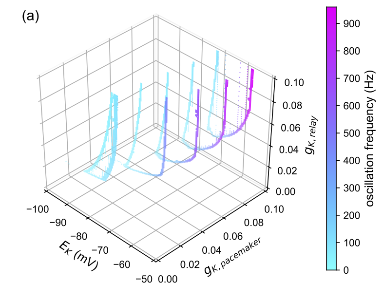
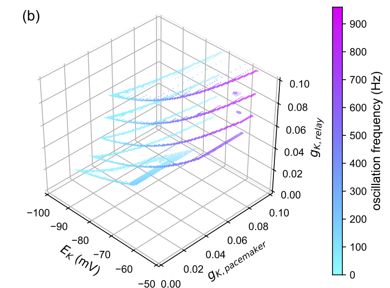