

Because I kept building new tools and functions for my linguistic research, I decided to put them together into
corpkit, a simple toolkit for working with parsed and structured linguistic corpora.Recently, I've been working on a GUI version of the tool. This resides as pure Python in
corpkit/corpkit-gui.py. There is also a zipped up version of an OSX executable in thecorpkit-appsubmodule. Documentation for the GUI is here. From here on out, though, this readme concerns the command line interface only.
- What's in here?
- Installation
- Unpacking the orientation data
- Quickstart
- More detailed examples
- More information
- Cite
Essentially, the module contains a bunch of functions for interrogating corpora, then manipulating or visualising the results. The most important of them are:
| Function name | Purpose |
|---|---|
interrogator() |
interrogate parse trees, dependencies, or find keywords or ngrams |
plotter() |
visualise interrogator() results with matplotlib |
conc() |
complex concordancing of subcorpora |
editor() |
edit interrogator() or conc() results, calculate keywords |
There are also some lists of words and dependency roles, which can be used to match systemic-functional process types. These are explained in more detail here.
While most of the tools are designed to work with corpora that are parsed (by e.g. Stanford CoreNLP) and structured (in a series of directories representing different points in time, speaker IDs, chapters of a book, etc.), the tools can also be used on text that is unparsed and/or unstructured. That said, you won't be able to do nearly as much cool stuff.
The idea is to run the tools from an IPython Notebook, but you could also operate the toolkit from the command line if you wanted to have less fun.
The most comprehensive use of corpkit to date has been for an investigation of the word risk in The New York Times, 1963–2014. The repository for that project is here; the Notebook demonstrating the use of corpkit can be viewed via either GitHub or NBviewer.
- Use Tregex or regular expressions to search parse trees or plain text for complex lexicogrammatical phenomena
- Search Stanford dependencies (whichever variety you like) for information about the role, governor, dependent or index of a token matching a regular expression
- Return words or phrases, POS/group/phrase tags, raw counts, or all three.
- Return lemmatised or unlemmatised results (using WordNet for constituency trees, and CoreNLP's lemmatisation for dependencies). Add words to
dictionaries/word_transforms.pymanually if need be - Look for keywords in each subcorpus (using code from Spindle), and chart their keyness
- Look for ngrams in each subcorpus, and chart their frequency
- Two-way UK-US spelling conversion (superior as the former may be), and the ability to add words manually
- Output Pandas DataFrames that can be easily edited and visualised
- Use parallel processing to search for a number of patterns, or search for the same pattern in multiple corpora
- Remove, keep or merge interrogation results or subcorpora using indices, words or regular expressions (see below)
- Sort results by name or total frequency
- Use linear regression to figure out the trajectories of results, and sort by the most increasing, decreasing or static values
- Show the p-value for linear regression slopes, or exclude results above p
- Work with absolute frequency, or determine ratios/percentage of another list:
- determine the total number of verbs, or total number of verbs that are be
- determine the percentage of verbs that are be
- determine the percentage of be verbs that are was
- determine the ratio of was/were ...
- etc.
- Plot more advanced kinds of relative frequency: for example, find all proper nouns that are subjects of clauses, and plot each word as a percentage of all instances of that word in the corpus (see below)
- Plot using Pandas/Matplotlib
- Interactive plots (hover-over text, interactive legends) using mpld3 (examples in the Risk Semantics notebook)
- Plot anything you like: words, tags, counts for grammatical features ...
- Create line charts, bar charts, pie charts, etc. with the
kindargument - Use
subplots = Trueto produce individual charts for each result - Customisable figure titles, axes labels, legends, image size, colormaps, etc.
- Use
TeXif you have it - Use log scales if you really want
- Use a number of chart styles, such as
ggplotorfivethirtyeight - Save images to file, as
.pdfor.png
- View top results as a table via
Pandas - Standalone tools for quickly and easily generating lists of keywords, ngrams, collocates and concordances
- Concordance using Tregex (i.e. concordance all nominal groups containing gross as an adjective with
NP < (JJ < /gross/)) - Randomise concordance results, determine window size, output to CSV, etc.
- Quickly save interrogations and figures to file, and reload results in new sessions with
save_result()andload_result() - Build dictionaries from corpora, subcorpora or concordance lines, which can then be used as reference corpora for keyword generation
- Start a new blank project with
new_project()
One of the main reasons for these tools was to make it quicker and easier to explore corpora in complex ways, using output from one tool as input for the next.
- n-gramming and keywording can be done via
interrogator() - keywording can easily be done on your concordance lines
- Use loops to concordance the top results from an interrogation, or check their keyness
- use
editor()to edit concordance line output as well as interrogations - build a dictionary from a corpus, subcorpus, or from concordance lines, and use it as a reference corpus for keywording
- Restrict keyword analysis to particular parts of lexis/grammar (i.e. NP heads), removing the need for stopword lists, and making topic summarisation easier
- Use
interrogator()output or subset of output as target or reference corpus - and so on ...
Included here is a sample project, orientation, which you can run in order to familiarise yourself with the corpkit module. It uses a corpus of paragraphs of the NYT containing the word risk. Due to size restrictions, This data only includes parse trees (no dependencies), and isn't included in the pip package.
You can get corpkit running by downloading or cloning this repository, or via pip.
Hit 'Download ZIP' and unzip the file. Then cd into the newly created directory and install:
cd corpkit-master
# might need sudo:
python setup.py installClone the repo, cd into it and run the setup:
git clone https://github.com/interrogator/corpkit.git
cd corpkit
# might need sudo:
python setup.py install# might need sudo:
pip install corpkitTo interrogate corpora and plot results, you need Java, NLTK and matplotlib. Dependency searching needs Beautiful Soup. Tabling results needs Pandas, etc. For NLTK, you can also use pip:
# might need sudo
pip install -U nltk
The pip installation of NLTK does not come with the data needed for NLTK's tokeniser, so you'll also need to install that from Python:
>>> import nltk
# change 'punkt' to 'all' to get everything
>>> nltk.download('punkt')If you installed by downloading or cloning this repository, you'll have the orientation project installed. To use it, cd into the orientation project and unzip the data files:
cd orientation
# unzip data to data folder
gzip -dc data/nyt.tar.gz | tar -xf - -C dataThe best way to use corpkit is by opening orientation.ipynb with IPython, and executing the first few cells:
ipython notebook orientation.ipynbOr, just use (I)Python (more difficult, less fun):
>>> import corpkit
>>> from corpkit import interroplot

# set corpus path
>>> corpus = 'data/nyt/years'

# search nyt for modal auxiliaries:
>>> interroplot(corpus, r'MD')
Output:
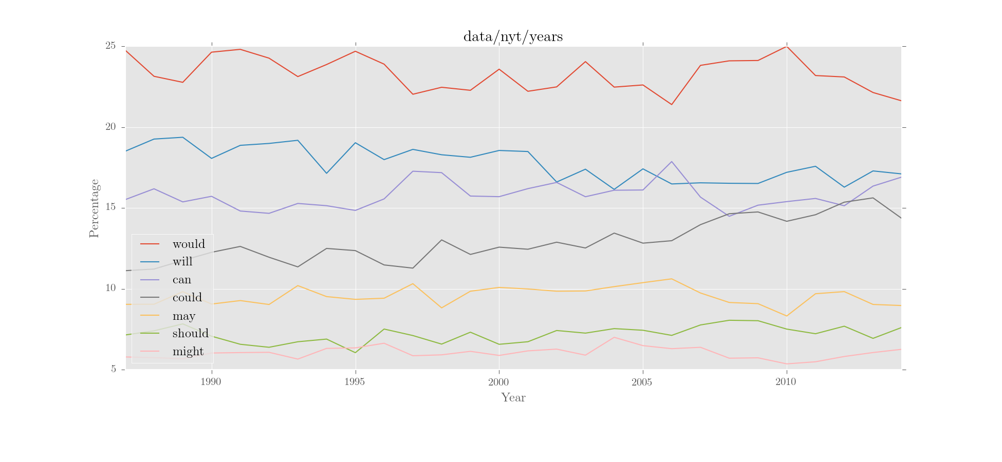
interroplot() is just a demo function that does three things in order:
- uses
interrogator()to search corpus for a (Regex or Tregex) query - uses
editor()to calculate the relative frequencies of each result - uses
plotter()to show the top seven results
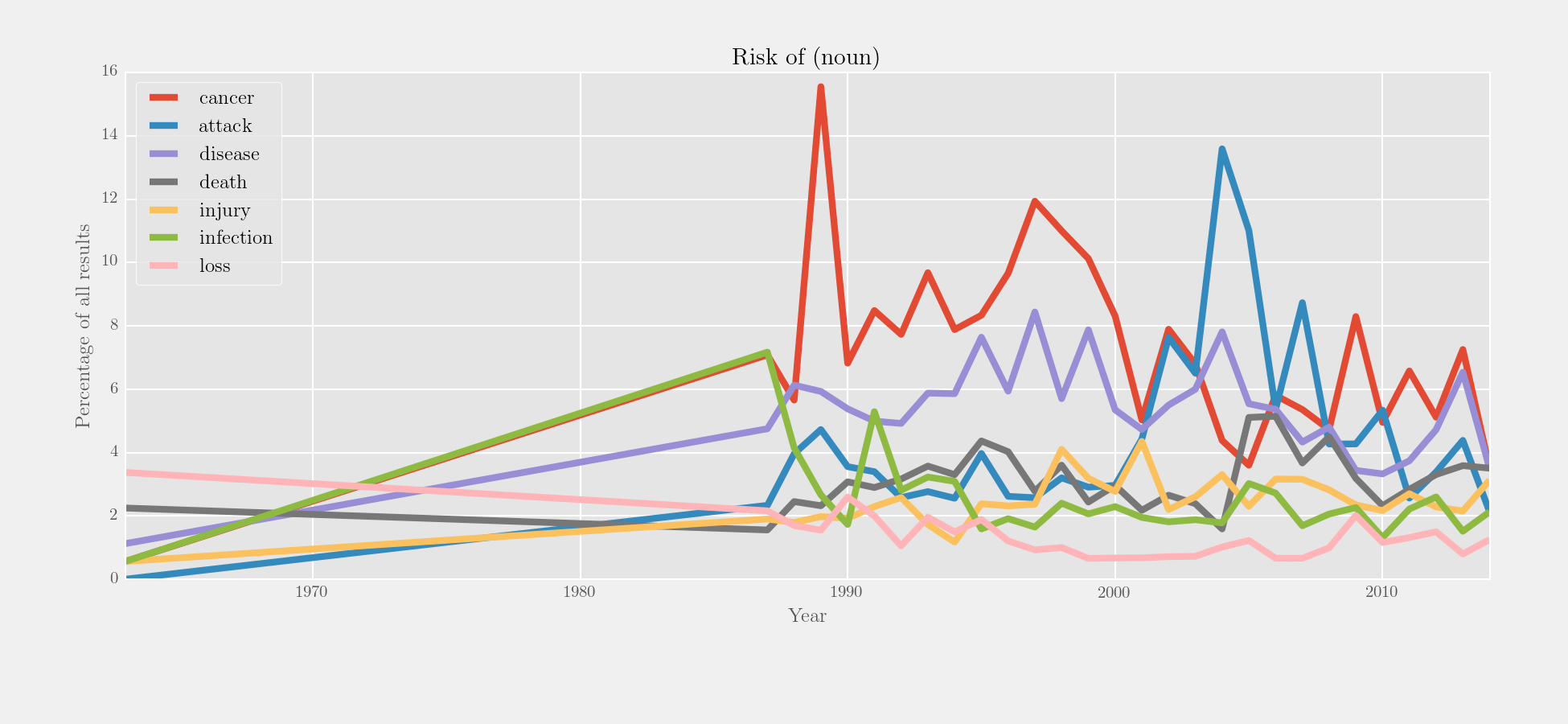
Here's an example of the three functions at work on the NYT corpus:
>>> from corpkit import interrogator, editor, plotter
# make tregex query: head of NP in PP containing 'of'
# in NP headed by risk word:
>>> q = r'/NN.?/ >># (NP > (PP <<# /(?i)of/ > (NP <<# (/NN.?/ < /(?i).?\brisk.?/))))'

# count terminals/leaves of trees only, and do lemmatisation:
>>> risk_of = interrogator(corpus, 'words', q, lemmatise = True)

# use editor to turn absolute into relative frequencies
>>> to_plot = editor(risk_of.results, '%', risk_of.totals)

# plot the results
>>> plotter('Risk of (noun)', to_plot.results, y_label = 'Percentage of all results',
...    style = 'fivethirtyeight')
Output:
You can use Tregex queries to concordance things, too:
>>> from corpkit import conc

>>> subcorpus = 'data/nyt/years/2005'
>>> query = r'/JJ.?/ > (NP <<# (/NN.?/ < /\brisk/))'
>>> lines = conc(subcorpus, query, window = 50, n = 10, random = True)
Output (a Pandas DataFrame):
0    hedge funds or high-risk stocks obviously poses a         greater   risk to the pension program than a portfolio of
1           contaminated water pose serious health and   environmental   risks
2   a cash break-even pace '' was intended to minimize       financial   risk to the parent company
3                                                Other           major   risks identified within days of the attack
4                           One seeks out stocks ; the           other   monitors risks
5        men and women in Colorado Springs who were at            high   risk for H.I.V. infection , because of
6   by the marketing consultant Seth Godin , to taking      calculated   risks , in the opinion of two longtime business
7        to happen '' in premises '' where there was a            high   risk of fire
8       As this was match points , some of them took a          slight   risk at the second trick by finessing the heart
9     said that the agency 's continuing review of how         Guidant   treated patient risks posed by devices like the
You can use this output as a dictionary, or extract keywords and ngrams from it, or keep or remove certain results with editor().
Because I mostly use systemic functional grammar, there is also a simple tool for distinguishing between process types (relational, mental, verbal) when interrogating a corpus. If you add words to the lists in dictionaries/process_types.py, pattern.en will get all their inflections automatically.
>>> from corpkit import quickview
>>> from dictionaries.process_types import processes

# use verbal process regex as the query
# deprole finds the dependent of verbal processes, and its functional role
# keep only results matching function_filter regex
>>> sayers = interrogator(corpus, 'd', processes.verbal,
...    function_filter = r'^nsubj$', lemmatise = True)

# have a look at the top results
>>> quickview(sayers, n = 20)
Output:
  0: he (n=24530)
  1: she (n=5558)
  2: they (n=5510)
  3: official (n=4348)
  4: it (n=3752)
  5: who (n=2940)
  6: that (n=2665)
  7: i (n=2062)
  8: expert (n=2057)
  9: analyst (n=1369)
 10: we (n=1214)
 11: report (n=1103)
 12: company (n=1070)
 13: which (n=1043)
 14: you (n=987)
 15: researcher (n=987)
 16: study (n=901)
 17: critic (n=826)
 18: person (n=802)
 19: agency (n=798)
 20: doctor (n=770)
First, let's try removing the pronouns using editor(). The quickest way is to use the editable wordlists stored in dictionaries/wordlists:
>>> from corpkit import editor
>>> from dictionaries.wordlists import wordlists
>>> prps = wordlists.pronouns

# alternative approaches:
# >>> prps = [0, 1, 2, 4, 5, 6, 7, 10, 13, 14, 24]
# >>> prps = ['he', 'she', 'you']
# >>> prps = as_regex(wl.pronouns, boundaries = 'line')

# give editor() indices, words, wordlists or regexes to keep remove or merge
>>> sayers_no_prp = editor(sayers.results, skip_entries = prps,
...    skip_subcorpora = [1963])
>>> quickview(sayers_no_prp, n = 10)
Output:
  0: official (n=4342)
  1: expert (n=2055)
  2: analyst (n=1369)
  3: report (n=1098)
  4: company (n=1066)
  5: researcher (n=987)
  6: study (n=900)
  7: critic (n=825)
  8: person (n=801)
  9: agency (n=796)
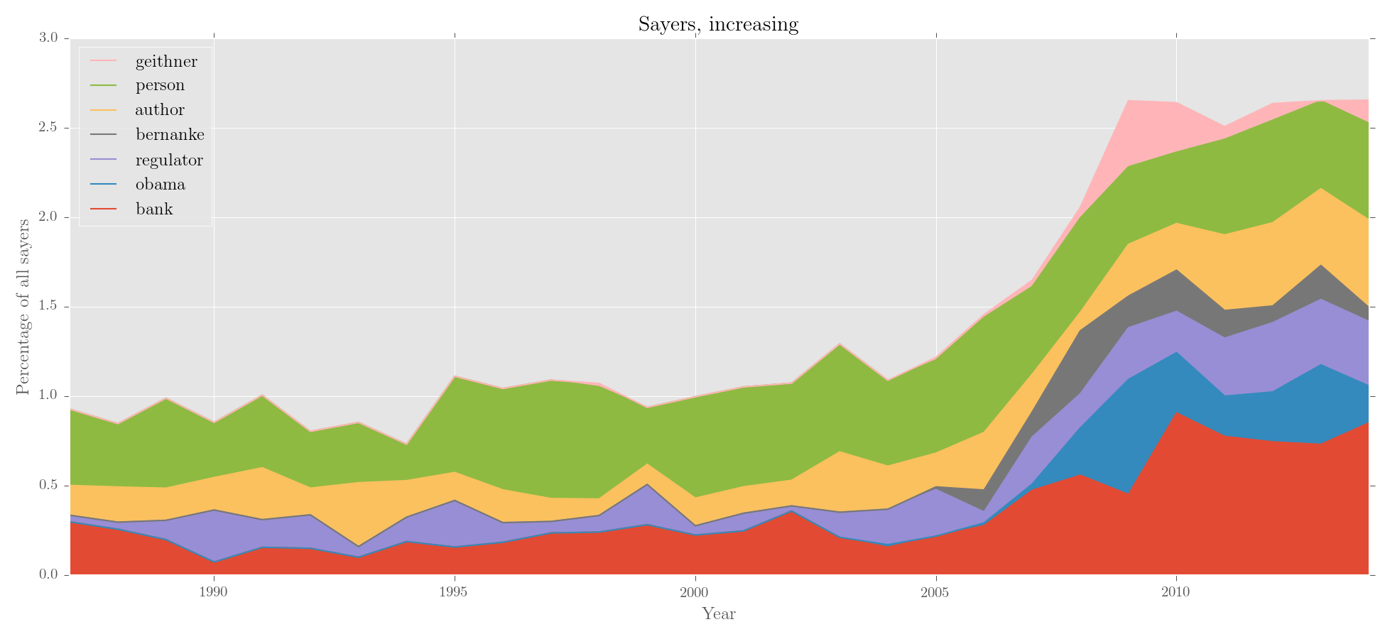
Great. Now, let's sort the entries by trajectory, and then plot:
# sort with editor()
>>> sayers_no_prp = editor(sayers_no_prp.results, '%', sayers.totals, sort_by = 'increase')

# make an area chart with custom y label
>>> plotter('Sayers, increasing', sayers_no_prp.results, kind = 'area',
...    y_label = 'Percentage of all sayers')
Output:
We can also merge subcorpora. Let's look for changes in gendered pronouns:
>>> subcorpora_to_merge = [('1960s', r'^196'),
...    ('1980s', r'^198'), ('1990s', r'^199'),
...    ('2000s', r'^200'), ('2010s', r'^201')]

>>> for subcorp, search in subcorpora_to_merge:
...    sayers = editor(sayers.results, merge_subcorpora = search, new_subcorpus_name=subcorp)

# now, get relative frequencies for he and she
>>> genders = editor(sayers.results, '%', sayers.totals, just_entries = ['he', 'she'])

# and plot it as a series of pie charts, showing totals on the slices:
>>> plotter('Pronominal sayers in the NYT', genders.results.T, kind = 'pie',
...    subplots = True, figsize = (15, 2.75), show_totals = 'plot')
Output:
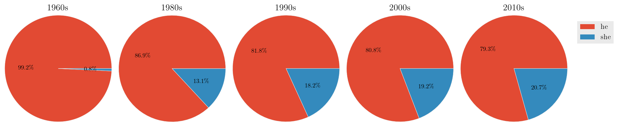
Woohoo, a decreasing gender divide!
As I see it, there are two main problems with keywording, as typically performed in corpus linguistics. First is the reliance on 'balanced'/'general' reference corpora, which are obviously a fiction. Second is the idea of stopwords. Essentially, when most people calculate keywords, they use stopword lists to automatically filter out words that they think will not be of interest to them. These words are generally closed class words, like determiners, prepositions, or pronouns. This is not a good way to go about things: the relative frequencies of I, you and one can tell us a lot about the kinds of language in a corpus. More seriously, stopwords mean adding subjective judgements about what is interesting language into a process that is useful precisely because it is not subjective or biased.
So, what to do? Well, first, don't use 'general reference corpora' unless you really really have to. With corpkit, you can use your entire corpus as the reference corpus, and look for keywords in subcorpora. Second, rather than using lists of stopwords, simply do not send all words in the corpus to the keyworder for calculation. Instead, try looking for key predicators (rightmost verbs in the VP), or key participants (heads of arguments of these VPs):
# just heads of participants (no pronouns, though!)
>>> part = r'/(NN|JJ).?/ >># (/(NP|ADJP)/ $ VP | > VP)'
>>> p = interrogator(corpus, 'words', part, lemmatise = True)
When using editor() to calculate keywords, there are a few default parameters that can be easily changed:
| Keyword argument | Function | Default setting | Type |
|---|---|---|---|
threshold |
Remove words occurring fewer than n times in reference corpus |
False |
'high/medium/low'/ True/False / int |
calc_all |
Calculate keyness for words in both reference and target corpus, rather than just target corpus | True |
True/False |
selfdrop |
Attempt to remove target data from reference data when calculating keyness | True |
True/False |
Let's have a look at how these options change the output:
# 'self' as reference corpus uses p.results
>>> options = {'selfdrop': True,
...            'selfdrop': False,
...            'calc_all': False,
...            'threshold': False}

>>> for k, v in options.items():
...    k = editor(p.results, 'keywords', 'self', k = v)
...    print k.results.ix['2011'].order(ascending = False)
Output:
| #1: default | #2: no selfdrop |
#3: no calc_all |
#4: no threshold |
||||
|---|---|---|---|---|---|---|---|
| risk | 1941.47 | risk | 1909.79 | risk | 1941.47 | bank | 668.19 |
| bank | 1365.70 | bank | 1247.51 | bank | 1365.70 | crisis | 242.05 |
| crisis | 431.36 | crisis | 388.01 | crisis | 431.36 | obama | 172.41 |
| investor | 410.06 | investor | 387.08 | investor | 410.06 | demiraj | 161.90 |
| rule | 316.77 | rule | 293.33 | rule | 316.77 | regulator | 144.91 |
| ... | ... | ... | ... | ||||
| clinton | -37.80 | tactic | -35.09 | hussein | -25.42 | clinton | -87.33 |
| vioxx | -38.00 | vioxx | -35.29 | clinton | -37.80 | today | -89.49 |
| greenspan | -54.35 | greenspan | -51.38 | vioxx | -38.00 | risky | -125.76 |
| bush | -153.06 | bush | -143.02 | bush | -153.06 | bush | -253.95 |
| yesterday | -162.30 | yesterday | -151.71 | yesterday | -162.30 | yesterday | -268.29 |
As you can see, slight variations on keywording give different impressions of the same corpus!
A key strength of corpkit's approach to keywording is that you can generate new keyword lists without re-interrogating the corpus. Let's use Pandas syntax to look for keywords in the past few years:
>>> yrs = ['2011', '2012', '2013', '2014']
>>> keys = editor(p.results.ix[yrs].sum(), 'keywords', p.results.drop(yrs),
...    threshold = False)
>>> print keys.results
Output:
bank          1795.24
obama          722.36
romney         560.67
jpmorgan       527.57
rule           413.94
dimon          389.86
draghi         349.80
regulator      317.82
italy          282.00
crisis         243.43
putin          209.51
greece         208.80
snowden        208.35
mf             192.78
adoboli        161.30
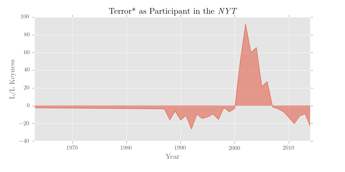
... or track the keyness of a set of words over time:
>>> terror = ['terror', 'terrorism', 'terrorist']
>>> terr = editor(p.results, 'k', 'self', merge_entries = terror, newname = 'terror')
>>> print terr.results.terror
Output:
1963    -2.51
1987    -3.67
1988   -16.09
1989    -6.24
1990   -16.24
...       ...
Name: terror, dtype: float64
Naturally, we can use plotter() for our keywords too:
>>> plotter('Terror* as Participant in the \emph{NYT}', pols.results.terror,
... kind = 'area', stacked = False, y_label = 'L/L Keyness')
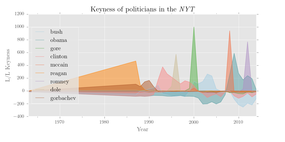
>>> politicians = ['bush', 'obama', 'gore', 'clinton', 'mccain',
... 'romney', 'dole', 'reagan', 'gorbachev']
>>> plotter('Keyness of politicians in the \emph{NYT}', k.results[politicans],
... num_to_plot = 'all', y_label = 'L/L Keyness', kind = 'area', legend_pos = 'center left')Output:
If you still want to use a standard reference corpus, you can do that (and a dictionary version of the BNC is included). For the reference corpus, editor() recognises dicts, DataFrames, Series, files containing dicts, or paths to plain text files or trees.
# arbitrary list of common/boring words
>>> from dictionaries.stopwords import stopwords
>>> print editor(p.results.ix['2013'], 'k', 'bnc.p',
...    skip_entries = stopwords).results
>>> print editor(p.results.ix['2013'], 'k', 'bnc.p', calc_all = False).results
Output (not so useful):
#1                                #2
bank           5568.25            bank      5568.25
person         5423.24            person    5423.24
company        3839.14            company   3839.14
way            3537.16            way       3537.16
state          2873.94            state     2873.94
                ...                           ...
three          -691.25            ten       -199.36
people         -829.97            bit       -205.97
going          -877.83            sort      -254.71
erm           -2429.29            thought   -255.72
yeah          -3179.90            will      -679.06
Finally, for the record, you could also use interrogator() or keywords() to calculate keywords, though these options may offer less flexibility:
>>> from corpkit import keywords
>>> keys = keywords(p.results.ix['2002'], reference_corpus = p.results])
>>> keys = interrogator(corpus, 'keywords', 'any', reference_corpus = 'self')interrogator() can also parallel-process multiple queries or corpora. Parallel processing will be automatically enabled if you pass in either:
- a
listof paths aspath(i.e.['path/to/corpus1', 'path/to/corpus2']) - a
dictasquery(i.e.{'Noun phrases': r'NP', 'Verb phrases': r'VP'})
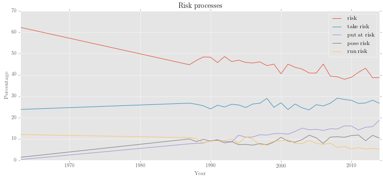
Let's look at different risk processes (e.g. risk, take risk, run risk, pose risk, put at risk) using constituency parses:
>>> query = {'risk': r'VP <<# (/VB.?/ < /(?i).?\brisk.?\b/)',
...    'take risk': r'VP <<# (/VB.?/ < /(?i)\b(take|takes|taking|took|taken)+\b/) < (NP <<# /(?i).?\brisk.?\b/)',
...    'run risk': r'VP <<# (/VB.?/ < /(?i)\b(run|runs|running|ran)+\b/) < (NP <<# /(?i).?\brisk.?\b/)',
...    'put at risk': r'VP <<# /(?i)(put|puts|putting)\b/ << (PP <<# /(?i)at/ < (NP <<# /(?i).?\brisk.?/))',
...    'pose risk': r'VP <<# (/VB.?/ < /(?i)\b(pose|poses|posed|posing)+\b/) < (NP <<# /(?i).?\brisk.?\b/)'}

>>> processes = interrogator(corpus, 'count', query)
>>> proc_rel = editor(processes.results, '%', processes.totals)
>>> plotter('Risk processes', proc_rel.results)
Output:
Next, let's find out what kinds of noun lemmas are subjects of any of these risk processes:
# a query to find heads of nps that are subjects of risk processes
>>> query = r'/^NN(S|)$/ !< /(?i).?\brisk.?/ >># (@NP $ (VP <+(VP) (VP ( <<# (/VB.?/ < /(?i).?\brisk.?/) ' \
...    r'| <<# (/VB.?/ < /(?i)\b(take|taking|takes|taken|took|run|running|runs|ran|put|putting|puts)/) < ' \
...    r'(NP <<# (/NN.?/ < /(?i).?\brisk.?/))))))'
>>> noun_riskers = interrogator(c, 'words', query, lemmatise = True)

>>> quickview(noun_riskers, 10)
Output:
  0: person (n=195)
  1: company (n=139)
  2: bank (n=80)
  3: investor (n=66)
  4: government (n=63)
  5: man (n=51)
  6: leader (n=48)
  7: woman (n=43)
  8: official (n=40)
  9: player (n=39)
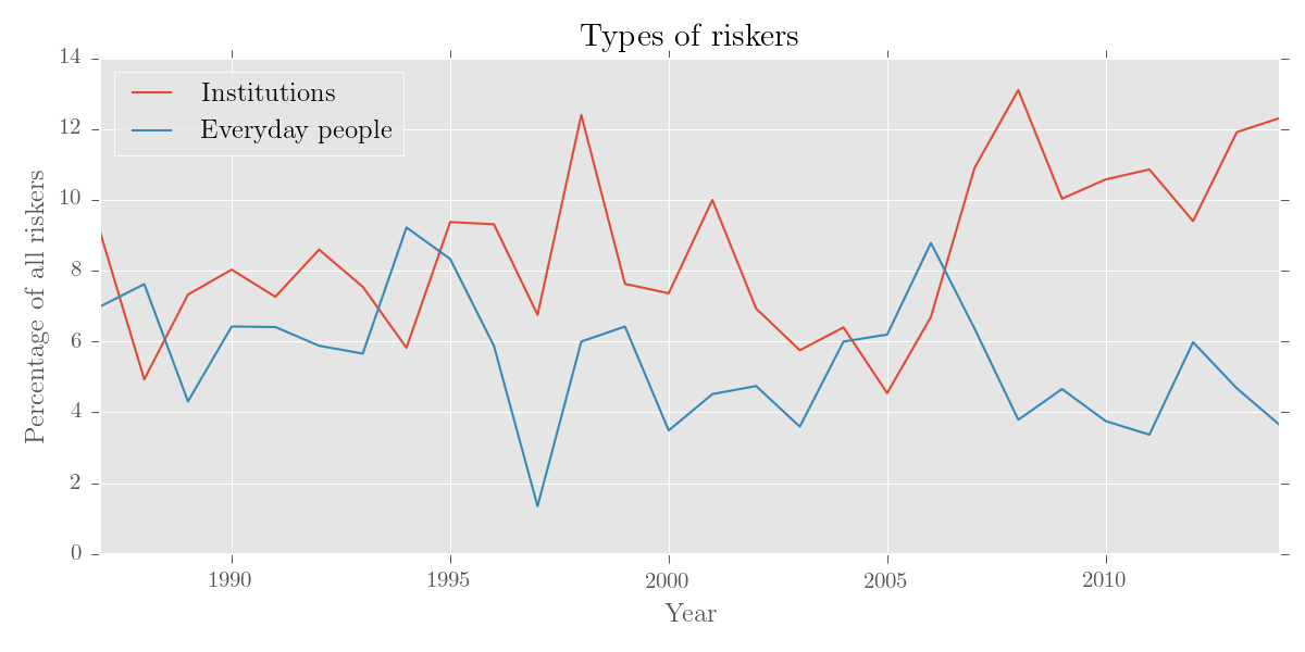
We can use editor() to make some thematic categories:
# get everyday people
>>> p = ['person', 'man', 'woman', 'child', 'consumer', 'baby', 'student', 'patient']

>>> them_cat = editor(noun_riskers.results, merge_entries = p, newname = 'Everyday people')

# get business, gov, institutions
>>> i = ['company', 'bank', 'investor', 'government', 'leader', 'president', 'officer',
...      'politician', 'institution', 'agency', 'candidate', 'firm']

>>> them_cat = editor(them_cat.results, '%', noun_riskers.totals, merge_entries = i,
...    newname = 'Institutions', sort_by = 'total', skip_subcorpora = 1963,
...    just_entries = ['Everyday people', 'Institutions'])

# plot result
>>> plotter('Types of riskers', them_cat.results, y_label = 'Percentage of all riskers')
Output:
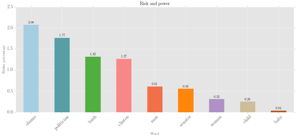
Let's also find out what percentage of the time some nouns appear as riskers:
# find any head of an np not containing risk
>>> query = r'/NN.?/ >># NP !< /(?i).?\brisk.?/'
>>> noun_lemmata = interrogator(corpus, 'words', query, lemmatise = True)

# get some key terms
>>> people = ['man', 'woman', 'child', 'baby', 'politician',
...           'senator', 'obama', 'clinton', 'bush']
>>> selected = editor(noun_riskers.results, '%', noun_lemmata.results,
...    just_entries = people, just_totals = True, threshold = 0, sort_by = 'total')

# make a bar chart:
>>> plotter('Risk and power', selected.results, num_to_plot = 'all', kind = 'bar',
...    x_label = 'Word', y_label = 'Risker percentage', fontsize = 15)
Output:
With a bit of creativity, you can do some pretty awesome data-viz, thanks to Pandas and Matplotlib. The following plots require only one interrogation:
>>> modals = interrogator(annual_trees, 'words', 'MD < __')
# simple stuff: make relative frequencies for individual or total results
>>> rel_modals = editor(modals.results, '%', modals.totals)

# trickier: make an 'others' result from low-total entries
>>> low_indices = range(7, modals.results.shape[1])
>>> each_md = editor(modals.results, '%', modals.totals, merge_entries = low_indices,
...    newname = 'other', sort_by = 'total', just_totals = True, keep_top = 7)

# complex stuff: merge results
>>> entries_to_merge = [r'(^w|\'ll|\'d)', r'^c', r'^m', r'^sh']
>>> for regex in entries_to_merge:
...    modals = editor(modals.results, merge_entries = regex)

# complex stuff: merge subcorpora
>>> subcorpora_to_merge = [('1960s', r'^196'), ('1980s', r'^198'), ('1990s', r'^199'),
...    ('2000s', r'^200'), ('2010s', r'^201')]
>>> for subcorp, search in subcorpora_to_merge:
...    modals = editor(modals.results, merge_subcorpora = search, new_subcorpus_name=subcorp)

# make relative, sort, remove what we don't want
>>> modals = editor(modals.results, '%', modals.totals, keep_stats = False,
...    just_subcorpora = [n for n, s in subcorpora_to_merge], sort_by = 'total', keep_top = 4)

# show results
>>> print rel_modals.results, each_md.results, modals.results
Output:
would will can could ... need shall dare shalt
1963 22.326833 23.537323 17.955615 6.590451 ... 0.000000 0.537996 0.000000 0
1987 24.750614 18.505132 15.512505 11.117537 ... 0.072286 0.260228 0.014457 0
1988 23.138986 19.257117 16.182067 11.219364 ... 0.091338 0.060892 0.000000 0
... ... ... ... ... ... ... ... ... ...
2012 23.097345 16.283186 15.132743 15.353982 ... 0.029499 0.029499 0.000000 0
2013 22.136269 17.286522 16.349301 15.620351 ... 0.029753 0.029753 0.000000 0
2014 21.618357 17.101449 16.908213 14.347826 ... 0.024155 0.000000 0.000000 0
[29 rows x 17 columns]
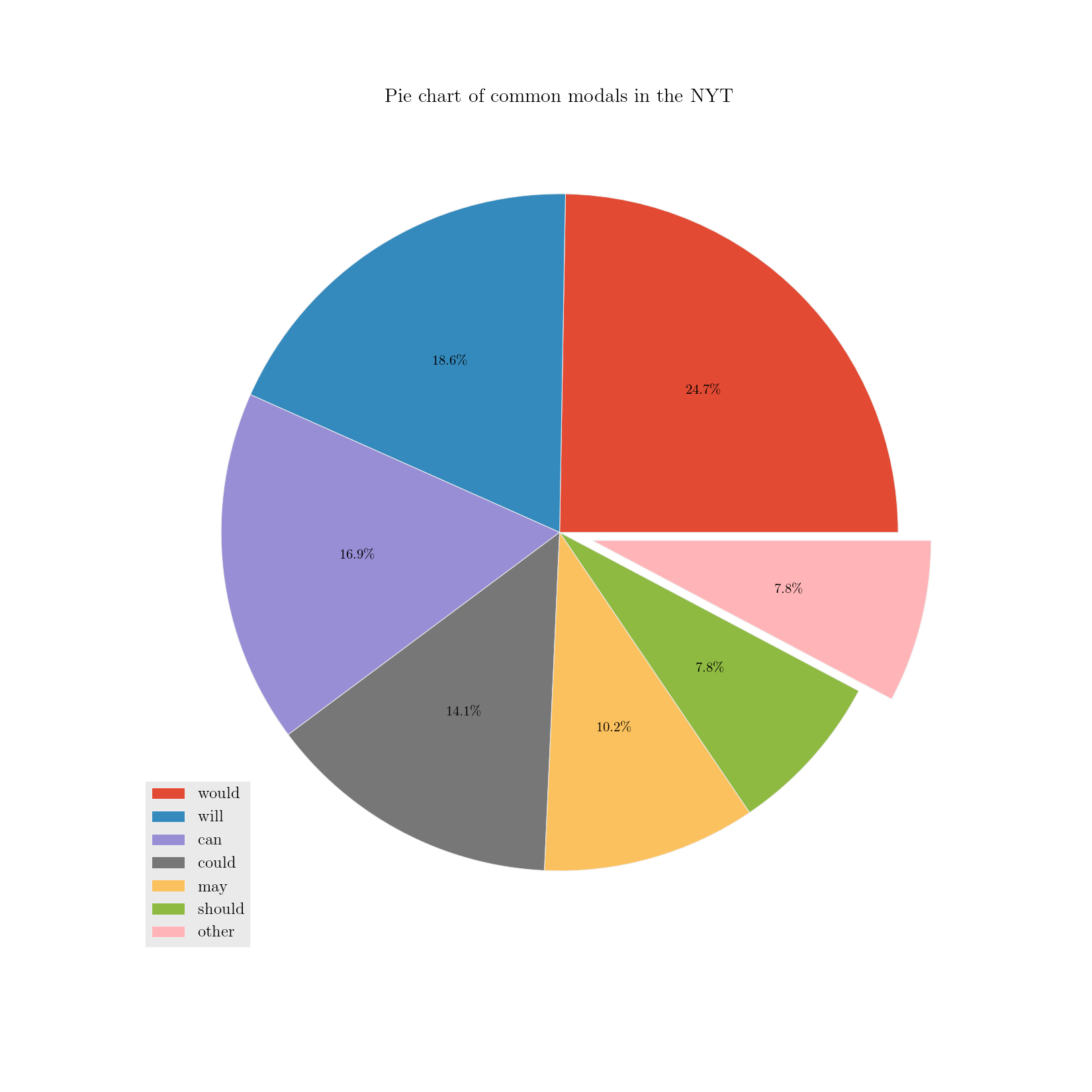
would 23.235853
will 17.484034
can 15.844070
could 13.243449
may 9.581255
should 7.292294
other 7.290155
Name: Combined total, dtype: float64
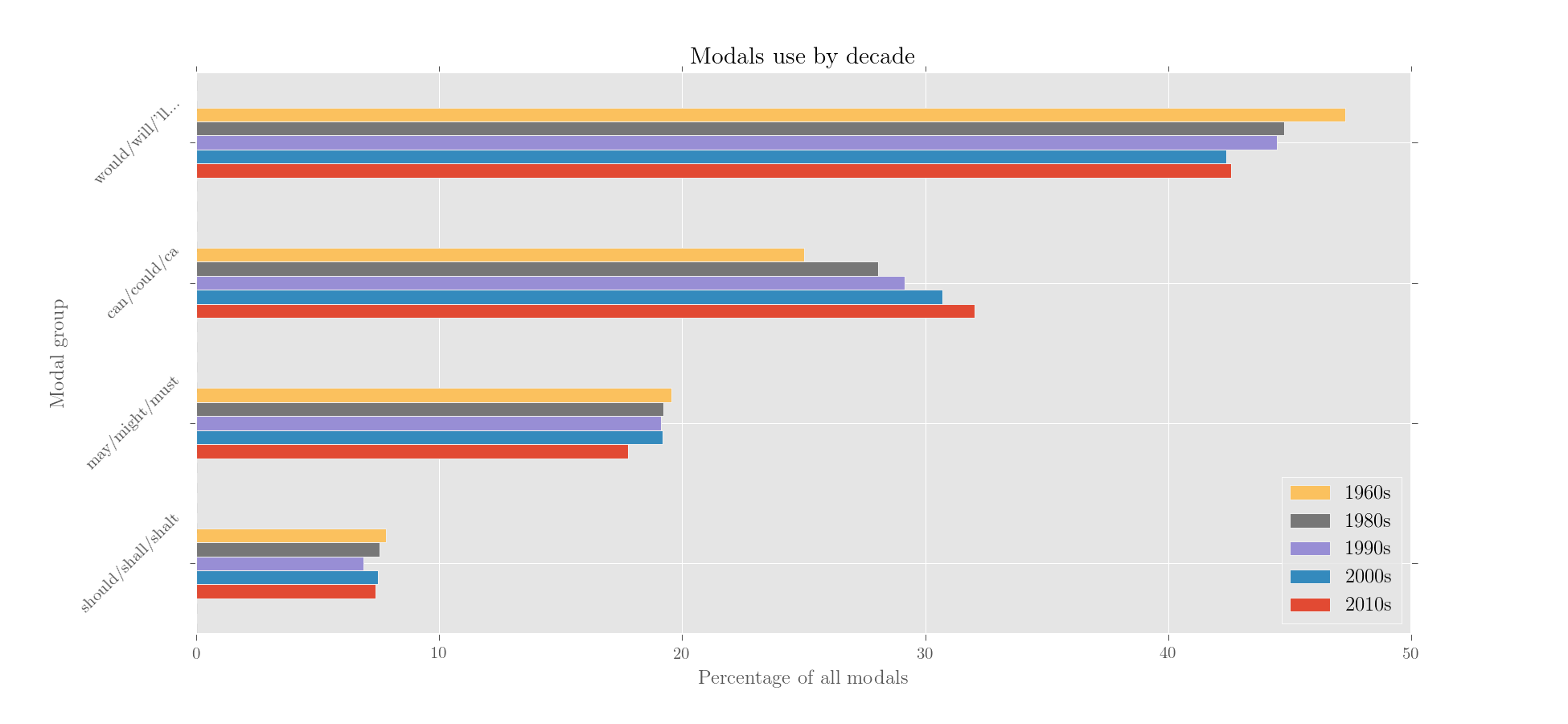
would/will/'ll... can/could/ca may/might/must should/shall/shalt
1960s 47.276395 25.016812 19.569603 7.800941
1980s 44.756285 28.050776 19.224476 7.566817
1990s 44.481957 29.142571 19.140310 6.892708
2000s 42.386571 30.710739 19.182867 7.485681
2010s 42.581666 32.045745 17.777845 7.397044
Now, some intense plotting:
# exploded pie chart
>>> plotter('Pie chart of common modals in the NYT', each_md.results, explode = ['other'],
... num_to_plot = 'all', kind = 'pie', colours = 'Accent', figsize = (11, 11))
# bar chart, transposing and reversing the data
>>> plotter('Modals use by decade', modals.results.iloc[::-1].T.iloc[::-1], kind = 'barh',
... x_label = 'Percentage of all modals', y_label = 'Modal group')
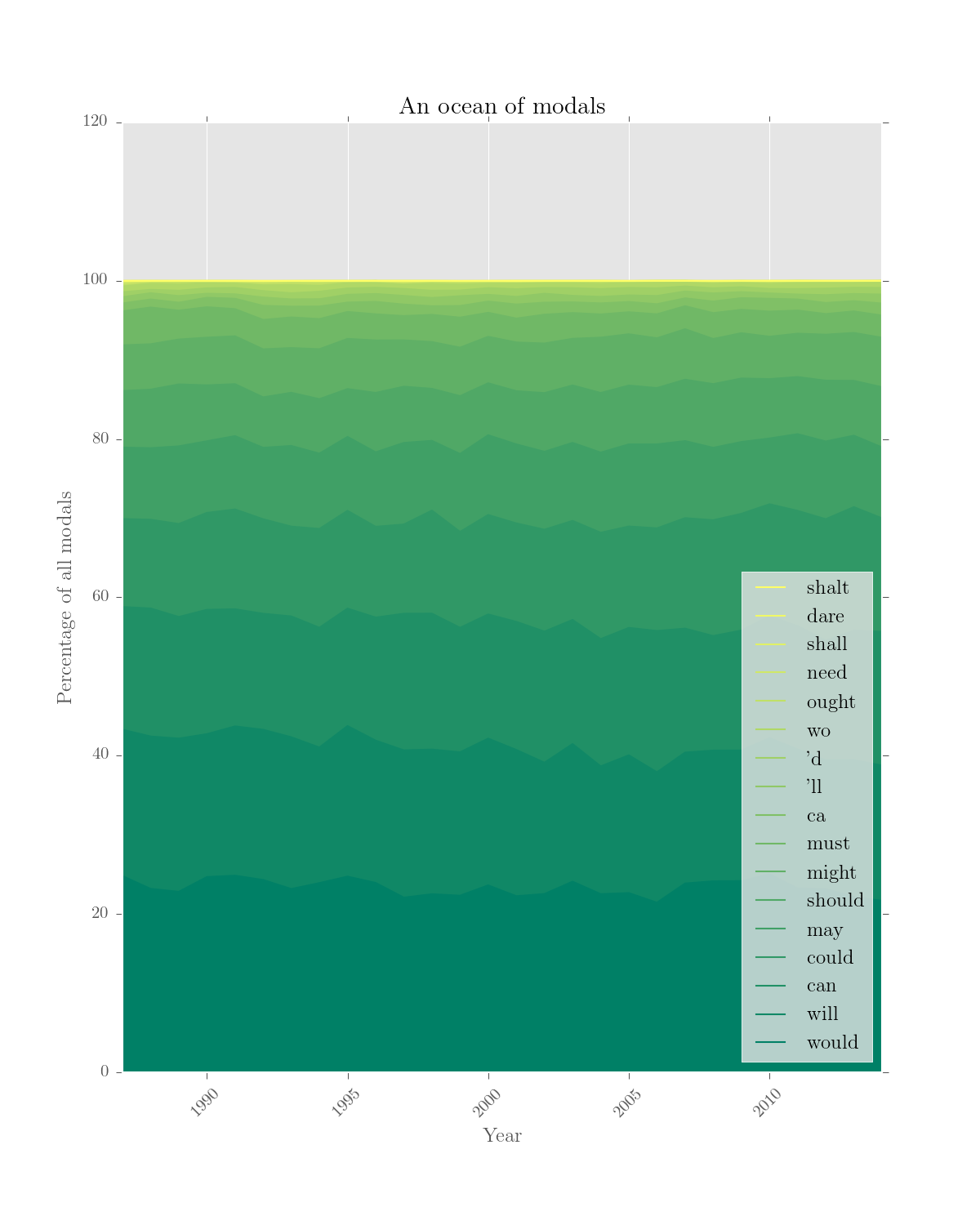
# stacked area chart
>>> plotter('An ocean of modals', rel_modals.results.drop('1963'), kind = 'area',
... stacked = True, colours = 'summer', figsize = (8, 10), num_to_plot = 'all',
... legend_pos = 'lower right', y_label = 'Percentage of all modals')Output:
Some things are likely lacking documentation right now. For now, the more complex functionality of the toolkit is presented best in some of the research projects I'm working on:
- Longitudinal linguistic change in an online support group (thesis project)
- Discourse-semantics of risk in the NYT, 1963–2014 (most
corpkituse) - Learning Python, IPython and NLTK by investigating a corpus of Malcolm Fraser's speeches
If you want to cite corpkit, please use:
McDonald, D. (2015). corpkit: a toolkit for corpus linguistics. Retrieved from https://www.github.com/interrogator/corpkit. DOI: http://doi.org/10.5281/zenodo.28361