 def saveToFile(self, outputfile) :
         myutil.log("save dump files to: " + outputfile)

         import io
         f = open(outputfile, 'w')
         for item in g_files.values():
                 item.printToFile(f)
         f.flush()
         f.close()
    def saveToFile(self, outputfile):
        myutil.log("save dump files to: " + outputfile)

        import io
        f = open(outputfile, 'w')
        for item in g_files.values():
            item.printToFile(f)
        f.flush()
        f.close()
 def testfolder(self):
         myutil.log2('test folder')
         import os
         folder = 'D:\\tech\\python\\Python33\\CodeCoverageHelper\\src\\Fusion\\Sketch\\Server\\Sketch\\ConstraintSolver'
         print("folder: " + folder)
         files = os.listdir(folder)
         for f in files:
                 ftmp = os.path.join(folder, f)
                 if os.path.isfile(ftmp):
                         myutil.log(f)
                         self.target.getClasses(ftmp)
from torch.utils.data import Dataset
import matplotlib.pyplot as plt  # 맷플롯립사용
import torchvision.datasets as dsets
import torchvision.transforms as transforms
from torch.utils.data import DataLoader
import random
from sklearn.datasets import load_digits

################################################################################
# - CNN으로 MNIST 분류하기
#   - 이번 챕터에서는 CNN으로 MNIST를 분류해보겠습니다.

################################################################################
# 임의의 텐서를 만듭니다. 텐서의 크기는 1 × 1 × 28 × 28입니다.
inputs = torch.Tensor(1, 1, 28, 28)
mu.log("inputs", inputs)

################################################################################
# - 합성곱층과 풀링 선언하기
#   - 이제 첫번째 합성곱 층을 구현해봅시다.
#   - 1채널 짜리를 입력받아서 32채널을 뽑아내는데 커널 사이즈는 3이고 패딩은 1입니다.
conv1 = nn.Conv2d(in_channels=1,
                  out_channels=32,
                  kernel_size=(3, 3),
                  padding=(1, 1))
mu.log("conv1", conv1)

################################################################################
# - 이제 두번째 합성곱 층을 구현해봅시다.
#   - 32채널 짜리를 입력받아서 64채널을 뽑아내는데 커널 사이즈는 3이고 패딩은 1입니다.
conv2 = nn.Conv2d(in_channels=32,
#   - 이번 챕터에서는 소프트맥스 회귀를 로우-레벨과 F.cross_entropy를 사용해서 구현해보겠습니다.

################################################################################
# - 소프트맥스 회귀 구현하기(로우-레벨)

torch.manual_seed(1)

x_train = [[1, 2, 1, 1], [2, 1, 3, 2], [3, 1, 3, 4], [4, 1, 5, 5],
           [1, 7, 5, 5], [1, 2, 5, 6], [1, 6, 6, 6], [1, 7, 7, 7]]

y_train = [2, 2, 2, 1, 1, 1, 0, 0]

x_train = torch.FloatTensor(x_train)
y_train = torch.LongTensor(y_train)

mu.log("x_train", x_train)
mu.log("y_train", y_train)

y_one_hot = torch.zeros(8, 3)
y_one_hot.scatter_(dim=1, index=y_train.unsqueeze(dim=1), value=1)
mu.log("y_one_hot", y_one_hot)

W = torch.zeros((4, 3), requires_grad=True)
b = torch.zeros(1, requires_grad=True)
optimizer = optim.SGD([W, b], lr=0.1)
nb_epoches = 2000
mu.plt_init()

for epoch in range(nb_epoches + 1):
    hypothesis = F.softmax(x_train.matmul(W) + b, dim=1)
    cost = (y_one_hot * -torch.log(hypothesis)).sum().mean()
# 학습에 사용할 파라미터를 설정합니다.

learning_rate = 0.001
training_epochs = 15
batch_size = 100

################################################################################
# 데이터로더를 사용하여 데이터를 다루기 위해서 데이터셋을 정의해줍니다.

mnist_train = dsets.MNIST(
    root='MNIST_data/',  # 다운로드 경로 지정
    train=True,  # True를 지정하면 훈련 데이터로 다운로드
    transform=transforms.ToTensor(),  # 텐서로 변환
    download=True)

mu.log("mnist_train", mnist_train)

mnist_test = dsets.MNIST(
    root='MNIST_data/',  # 다운로드 경로 지정
    train=False,  # False를 지정하면 테스트 데이터로 다운로드
    transform=transforms.ToTensor(),  # 텐서로 변환
    download=True)

mu.log("mnist_test", mnist_test)

data_loader = torch.utils.data.DataLoader(dataset=mnist_train,
                                          batch_size=batch_size,
                                          shuffle=True,
                                          drop_last=True)

mu.log("len(data_loader)", len(data_loader))
def printresult(res):
        logging.debug("results")
        for i in res:
                myutil.log(i)
import torch.nn as nn
import torch.nn.functional as F
import torch.optim as optim
from torch.utils.data import TensorDataset  # 텐서데이터셋
from torch.utils.data import DataLoader  # 데이터로더
from torch.utils.data import Dataset
import matplotlib.pyplot as plt  # 맷플롯립사용

################################################################################
# - 파이토치로 소프트맥스의 비용 함수 구현하기 (로우-레벨)

torch.manual_seed(1)

z = torch.FloatTensor([1, 2, 3])
hypothesis = F.softmax(z, dim=0)
mu.log("z", z)
mu.log("hypothesis", hypothesis)
mu.log("hypothesis.sum()", hypothesis.sum())

z = torch.rand(3, 5, requires_grad=True)
mu.log("z", z)
hypothesis = F.softmax(z, dim=1)
mu.log("hypothesis", hypothesis)
mu.log("hypothesis.sum(dim=1)", hypothesis.sum(dim=1))

y = torch.randint(5, (3, ))
mu.log("y", y)
hypothesis = F.softmax(z, dim=1)
mu.log("hypothesis", hypothesis)
y_one_hot = torch.zeros_like(hypothesis)
mu.log("y_one_hot", y_one_hot)
################################################################################
# - NLP에서의 원-핫 인코딩(One-hot encoding)
#   - 우선, 한국어 자연어 처리를 위해 코엔엘파이 패키지를 설치합니다.
#
# ```
# pip install konlpy
# ```
#
#   - 코엔엘파이의 Okt 형태소 분석기를 통해서 우선 문장에 대해서 토큰화를 수행하였습니다.

from konlpy.tag import Okt

okt = Okt()
token = okt.morphs("나는 자연어 처리를 배운다")
mu.log("token", token)
word2index = {}

for voca in token:
    if voca not in word2index.keys():
        word2index[voca] = len(word2index)

mu.log("word2index", word2index)

################################################################################
# - 토큰을 입력하면 해당 토큰에 대한 원-핫 벡터를 만들어내는 함수를 만들었습니다.


def one_hot_encoding(word, word2index):
    one_hot_vector = [0] * len(word2index)
    index = word2index[word]
Y = torch.FloatTensor([[0], [1], [1], [0]]).to(device)
################################################################################
# 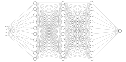
model = nn.Sequential(
nn.Linear(2, 10, bias=True), # input_layer = 2, hidden_layer1 = 10
nn.Sigmoid(),
nn.Linear(10, 10, bias=True), # hidden_layer1 = 10, hidden_layer2 = 10
nn.Sigmoid(),
nn.Linear(10, 10, bias=True), # hidden_layer2 = 10, hidden_layer3 = 10
nn.Sigmoid(),
nn.Linear(10, 1, bias=True), # hidden_layer3 = 10, output_layer = 1
nn.Sigmoid()).to(device)
mu.log("model", model)
################################################################################
# - 이제 비용 함수와 옵타마이저를 선언합니다.
# - nn.BCELoss()는 이진 분류에서 사용하는 크로스엔트로피 함수입니다.
criterion = nn.BCELoss().to(device)
optimizer = optim.SGD(model.parameters(), lr=1)
nb_epochs = 10000
mu.plt_init()
for epoch in range(nb_epochs):
hypothesis = model(X)
cost = criterion(hypothesis, Y)
optimizer.zero_grad()
cost.backward()
# - y 의 실제값이 1일 때 −logH(x) 그래프를 사용하고
# - y의 실제값이 0일 때 −log(1−H(X)) 그래프를 사용해야 합니다.
# - 이는 다음과 같이 하나의 식으로 통합할 수 있습니다.
#  = -\frac{1}{n} \sum_{i=1}^{n} [y^{(i)}logH(x^{(i)}) %2B (1-y^{(i)})log(1-H(x^{(i)}))])
torch.manual_seed(1)
x_data = [[1, 2], [2, 3], [3, 1], [4, 3], [5, 3], [6, 2]]
y_data = [[0], [0], [0], [1], [1], [1]]
x_train = torch.FloatTensor(x_data)
y_train = torch.FloatTensor(y_data)
W = torch.zeros((2, 1), requires_grad=True)
b = torch.zeros(1, requires_grad=True)
hypothesis = 1 / (1 + torch.exp(-(x_train.matmul(W) + b)))
mu.log("hypothesis", hypothesis)
mu.log("y_train", y_train)
hypothesis = torch.sigmoid(x_train.matmul(W) + b)
mu.log("hypothesis", hypothesis)
mu.log("y_train", y_train)
losses = -(y_train *
torch.log(hypothesis)) + (1 - y_train) * torch.log(1 - hypothesis)
cost = losses.mean()
mu.log("losses", losses)
mu.log("cost", cost)
loss = F.binary_cross_entropy(hypothesis, y_train)
mu.log("loss.item()", loss.item())
#
# 
################################################################################
# - 파이썬으로 RNN 구현하기
# - 직접 Numpy로 RNN 층을 구현해보겠습니다. 앞서 메모리 셀에서 은닉 상태를 계산하는 식을 다음과 같이 정의하였습니다.
# - ht=tanh(WxXt+Whht−1+b)
import numpy as np
timesteps = 10
input_size = 4
hidden_size = 8
inputs = np.random.random((timesteps, input_size))
mu.log("inputs.shape", inputs.shape)
hidden_state_t = np.zeros((hidden_size, ))
mu.log("hidden_state_t.shape", hidden_state_t.shape)
Wx = np.random.random((hidden_size, input_size))
Wh = np.random.random((hidden_size, hidden_size))
b = np.random.random((hidden_size, ))
mu.log("Wx.shape", Wx.shape)
mu.log("Wh.shape", Wh.shape)
mu.log("b.shape", b.shape)
total_hidden_states = []
# 메모리 셀 동작
# - 결과적으로 nn.Linear()의 결과를 nn.Sigmoid()를 거치게하면
# - 로지스틱 회귀의 가설식이 됩니다.
"""

lineArray = multi_lines.splitlines()

torch.manual_seed(1)

x_data = [[1, 2], [2, 3], [3, 1], [4, 3], [5, 3], [6, 2]]
y_data = [[0], [0], [0], [1], [1], [1]]
x_train = torch.FloatTensor(x_data)
y_train = torch.FloatTensor(y_data)

model = nn.Sequential(nn.Linear(2, 1), nn.Sigmoid())

mu.log("model", model)
mu.log("model(x_train)", model(x_train))

optimizer = optim.SGD(model.parameters(), lr=1)
nb_epoches = 1000

plt_epoch = []
plt_accuracy = []
mu.plt_init()

for epoch in range(nb_epoches + 1):
    hypothesis = model(x_train)
    cost = F.binary_cross_entropy(hypothesis, y_train)
    optimizer.zero_grad()
    cost.backward()
    optimizer.step()
#   - 자연어 처리는 일반적으로 토큰화, 단어 집합 생성, 정수 인코딩, 패딩, 벡터화의 과정을 거칩니다.
#   - 이번 챕터에서는 이러한 전반적인 과정에 대해서 이해합니다.

################################################################################
# - spaCy 사용하기
#
# ```
# pip install spacy
# python3 -m spacy download en
# ```

import spacy

en_text = "A Dog Run back corner near spare bedrooms"
spacy_en = spacy.load("en")
mu.log("spacy_en", spacy_en)


def tokenize(en_text):
    return [tok.text for tok in spacy_en.tokenizer(en_text)]


mu.log("tokenize(en_text)", tokenize(en_text))

################################################################################
# - NLTK 사용하기
#
# ```
# pip install nltk
# ```
#
    cost = torch.mean((hypothesis - y_train)**2)

    # accuracy 계산
    accuracy = mu.get_regression_accuracy(hypothesis, y_train)

    # cost로 H(x) 개선
    optimizer.zero_grad()
    cost.backward()
    optimizer.step()

    # 100번마다 로그 출력
    if epoch % 100 == 0:
        mu.log_epoch(epoch, nb_epochs, cost, accuracy)

mu.plt_show()
mu.log("W", W)
mu.log("b", b)

################################################################################
# optimizer.zero_grad()가 필요한 이유

import torch

w = torch.tensor(2.0, requires_grad=True)

nb_epochs = 20
for epoch in range(nb_epochs + 1):
    z = 2 * w

    z.backward()
    print('수식을 w로 미분한 값 : {}'.format(w.grad))
import torchvision.datasets as dsets
import torchvision.transforms as transforms
from torch.utils.data import DataLoader
import random

################################################################################
# - 소프트맥스 회귀로 MNIST 데이터 분류하기
#   - 이번 챕터에서는 MNIST 데이터에 대해서 이해하고,
#   - 파이토치(PyTorch)로 소프트맥스 회귀를 구현하여 MNIST 데이터를 분류하는 실습을 진행해봅시다.

################################################################################
# 현재 환경에서 GPU 연산이 가능하다면 GPU 연산을 하고, 그렇지 않다면 CPU 연산을 하도록 합니다.

USE_CUDA = torch.cuda.is_available()
device = torch.device("cuda" if USE_CUDA else "cpu")
mu.log("device", device)

random.seed(777)
torch.manual_seed(777)

if device == "cuda":
    torch.cuda.manual_seed_all(777)

################################################################################
# - 하이퍼파라미터를 변수로 둡니다.

traning_epochs = 15
batch_size = 100

################################################################################
# - MNIST 분류기 구현하기
import myutil as mu
import numpy as np
import torch

################################################################################
# 넘파이로 텐서 만들기(벡터와 행렬 만들기)

t = np.array([0., 1., 2., 3., 4., 5., 6.])
mu.log("t", t)
mu.log("t.ndim", t.ndim)
mu.log("t.shape", t.shape)
mu.log("t[-1]", t[-1])
mu.log("t[2:5]", t[2:5])
mu.log("t[4:-1]", t[4:-1])
mu.log("t[:2]", t[:2])
mu.log("t[3:]", t[3:])

t = np.array([[1., 2., 3.], [4., 5., 6.], [7., 8., 9.], [10., 11., 12.]])
mu.log("t", t)
mu.log("t.ndim", t.ndim)
mu.log("t.shape", t.shape)

t = torch.FloatTensor([0., 1., 2., 3., 4., 5., 6.])
mu.log("t", t)
mu.log("t.ndim", t.ndim)
mu.log("t.shape", t.shape)

################################################################################
# 파이토치 텐서 선언하기(PyTorch Tensor Allocation)

t = torch.FloatTensor([[1., 2., 3.], [4., 5., 6.], [7., 8., 9.],
x_train = torch.FloatTensor([[73, 80, 75], [93, 88, 93], [89, 91, 90],
                             [96, 98, 100], [73, 66, 70]])

y_train = torch.FloatTensor([[152], [185], [180], [196], [142]])

dataset = TensorDataset(x_train, y_train)
dataloader = DataLoader(dataset, batch_size=2, shuffle=True)
model = nn.Linear(3, 1)
optimizer = optim.SGD(model.parameters(), lr=1e-5)
nb_epoches = 20
mu.plt_init()

for epoch in range(nb_epoches + 1):
    print("=" * 80)

    for batch_idx, samples in enumerate(dataloader):
        print("-" * 80)
        print("-" * 80)
        mu.log("batch_idx", batch_idx)
        mu.log("samples", samples)
        prediction = model(x_train)
        cost = F.mse_loss(prediction, y_train)
        accuracy = mu.get_regression_accuracy(prediction, y_train)
        optimizer.zero_grad()
        cost.backward()
        optimizer.step()
        mu.log_epoch(epoch, nb_epoches, cost, accuracy)

mu.plt_show()
mu.log("model", model)
        return res


torch.manual_seed(1)

model = BinaryClassifier()
optimizer = optim.SGD(model.parameters(), lr=1)
nb_epoches = 1000

x_data = [[1, 2], [2, 3], [3, 1], [4, 3], [5, 3], [6, 2]]
y_data = [[0], [0], [0], [1], [1], [1]]
x_train = torch.FloatTensor(x_data)
y_train = torch.FloatTensor(y_data)

mu.plt_init()

for epoch in range(nb_epoches + 1):
    hypothesis = model(x_train)
    cost = F.binary_cross_entropy(hypothesis, y_train)
    optimizer.zero_grad()
    cost.backward()
    optimizer.step()

    if epoch % 100 == 0:
        accuracy = mu.get_binary_classification_accuracy(hypothesis, y_train)
        mu.log_epoch(epoch, nb_epoches, cost, accuracy)

mu.plt_show()
mu.log("model", model)
################################################################################
#


import urllib.request
import pandas as pd

if not os.path.isfile(".IMDb_Reviews.csv"):
    urllib.request.urlretrieve(
        url="https://raw.githubusercontent.com/LawrenceDuan/IMDb-Review-Analysis/master/IMDb_Reviews.csv",
        filename=".IMDb_Reviews.csv")

df = pd.read_csv(".IMDb_Reviews.csv", encoding="latin1")

mu.log("len(df)", len(df))
mu.log("df[:5]", df[:5])

train_df = df[:2500]
test_df = df[2500:]

train_df.to_csv(".train_data.csv", index=False)
test_df.to_csv(".test_data.csv", index=False)

################################################################################
#

from torchtext import data

TEXT = torchtext.data.Field(
    sequential=True,
    urllib.request.urlretrieve(
        url="https://raw.githubusercontent.com/GaoleMeng/RNN-and-FFNN-textClassification/master/ted_en-20160408.xml",
        filename=".ted_en-20160408.xml"
    )

################################################################################
# - 훈련 데이터 전처리하기

targetXML = open(
    file=".ted_en-20160408.xml",
    mode="r",
    encoding="UTF8")

target_text = etree.parse(targetXML)
target_text_xpath = target_text.xpath('//content/text()')
mu.log("len(target_text_xpath)", len(target_text_xpath))
mu.log("target_text_xpath[:5]", target_text_xpath[:5])

parse_text = "\n".join(target_text_xpath)
mu.log("len(parse_text)", len(parse_text))
mu.log("parse_text", parse_text[:300])

# 정규 표현식의 sub 모듈을 통해
# content 중간에 등장하는 (Audio), (Laughter) 등의 배경음 부분을 제거.
content_text = re.sub(r'\([^)]*\)', '', parse_text)
mu.log("len(content_text)", len(content_text))
mu.log("content_text", content_text[:300])

# 입력 코퍼스에 대해서 NLTK를 이용하여 문장 토큰화를 수행.
sent_text = sent_tokenize(content_text)
mu.log("len(sent_text)", len(sent_text))
def printresult(res):
    myutil.log("print files")
    for item in res.values():
        item.print()
import myutil as mu
import numpy as np
import torch

################################################################################
# 뷰(View) - 원소의 수를 유지하면서 텐서의 크기 변경. 매우 중요함!!

t = np.array([[[0, 1, 2], [3, 4, 5]], [[6, 7, 8], [9, 10, 11]]])

ft = torch.FloatTensor(t)
mu.log("t.shape", t.shape)
mu.log("ft.shape", ft.shape)

################################################################################
# 3차원 텐서에서 2차원 텐서로 변경

mu.log("ft.view([-1, 3])", ft.view([-1, 3]))
mu.log("ft.view([-1, 3]).shape", ft.view([-1, 3]).shape)

################################################################################
# 3차원 텐서의 크기 변경
mu.log("ft.view([-1, 1, 3])", ft.view([-1, 1, 3]))
mu.log("ft.view([-1, 1, 3]).shape", ft.view([-1, 1, 3]).shape)

################################################################################
# 스퀴즈(Squeeze) - 1인 차원을 제거한다.
ft = torch.FloatTensor([[0], [1], [2]])
mu.log("ft", ft)
mu.log("ft.shape", ft.shape)

################################################################################
def printresult(res):
        myutil.log("print files")
        for item in res.values():
                item.print()
################################################################################
#
#
# - LSTM(Long Short-Term Memory)
# - LSTM은 은닉층의 메모리 셀에 입력 게이트, 망각 게이트, 출력 게이트를 추가하여
# - 불필요한 기억을 지우고, 기억해야할 것들을 정합니다.
# - 요약하면 LSTM은 은닉 상태(hidden state)를 계산하는 식이 전통적인 RNN보다 조금 더 복잡해졌으며
# - 셀 상태(cell state)라는 값을 추가하였습니다.
# - 위의 그림에서는 t시점의 셀 상태를 Ct로 표현하고 있습니다.
# - LSTM은 RNN과 비교하여 긴 시퀀스의 입력을 처리하는데 탁월한 성능을 보입니다.
#
#
# 
import numpy as np
import torch
import torch.nn as nn
inputs = torch.Tensor(1, 10, 5)
cell = nn.LSTM(input_size=5,
hidden_size=8,
num_layers=2,
batch_first=True,
bidirectional=True)
outputs, _status = cell(inputs)
mu.log("_status", _status)
mu.log("outputs.shape", outputs.shape)
device = "cuda" if torch.cuda.is_available() else "cpu"
torch.manual_seed(777)

if device == "cuda":
    torch.cuda.manual_seed_all(777)

X = torch.FloatTensor([[0, 0], [0, 1], [1, 0], [1, 1]]).to(device)
Y = torch.FloatTensor([[0], [1], [1], [0]]).to(device)

model = nn.Sequential(
    nn.Linear(2, 1, bias=True),
    nn.Sigmoid()
).to(device)

mu.log("model", model)
nb_epochs = 1000
mu.plt_init()
criterion = nn.BCELoss().to(device)
optimizer = optim.SGD(model.parameters(), lr=1)

for epoch in range(nb_epochs + 1):
    hypothesis = model(X)
    cost = criterion(hypothesis, Y)
    optimizer.zero_grad()
    cost.backward()
    optimizer.step()

    if epoch % 100 == 0:
        accuracy = mu.get_binary_classification_accuracy(hypothesis, Y)
        mu.log_epoch(epoch, nb_epochs, cost, accuracy)
    cost = torch.mean((hypothesis - y_train)**2)

    # accuracy 계산
    accuracy = mu.get_regression_accuracy(hypothesis, y_train)

    # cost로 H(x) 개선
    optimizer.zero_grad()
    cost.backward()
    optimizer.step()

    # 100번마다 로그 출력
    if epoch % 100 == 0:
        mu.log_epoch(epoch, nb_epochs, cost, accuracy)

mu.plt_show()
mu.log("w1", w1)
mu.log("w2", w2)
mu.log("w3", w3)
mu.log("b", b)

################################################################################
# 벡터와 행렬 연산으로 바꾸기

x_train = torch.FloatTensor([[73, 80, 75], [93, 88, 93], [89, 91, 90],
                             [96, 98, 100], [73, 66, 70]])

y_train = torch.FloatTensor([[152], [185], [180], [196], [142]])

mu.log("x_train.shape", x_train.shape)
mu.log("y_train.shape", y_train.shape)
################################################################################
# - 다층 퍼셉트론으로 손글씨 분류하기
#   - 이번 챕터에서는 다층 퍼셉트론을 구현하고, 딥 러닝을 통해서 숫자 필기 데이터를 분류해봅시다.
#   - MNIST 데이터랑 다른 데이터입니다.

################################################################################
# - 숫자 필기 데이터 소개
#   - 숫자 필기 데이터는 사이킷런 패키지에서 제공하는 분류용 예제 데이터입니다.
#   - 0부터 9까지의 숫자를 손으로 쓴 이미지 데이터로 load_digits() 명령으로 로드할 수 있습니다.
#   - 각 이미지는 0부터 15까지의 명암을 가지는 8 × 8 = 64 픽셀 해상도의 흑백 이미지입니다.
#   - 그리고 해당 이미지가 1,797개가 있습니다.
#   - load_digits()를 통해 이미지 데이터를 로드할 수 있습니다.
#   - 로드한 전체 데이터를 digits에 저장합니다.

digits = load_digits()
mu.log("len(digits.images)", len(digits.images))

images_labels = list(zip(digits.images, digits.target))
sub_sample_size = 20

for i, (image, label) in enumerate(images_labels[:sub_sample_size]):
    plt.subplot(4, 5, i + 1)
    plt.axis("off")
    plt.imshow(image, cmap=plt.cm.gray_r, interpolation="nearest")
    plt.title("label : {}".format(label))

plt.show()

################################################################################
# - 다층 퍼셉트론 분류기 만들기
